4.4 sklearn实战：鸢尾花分类与房价预测

sklearn实战：鸢尾花分类与房价预测

两个完整项目，从数据加载到模型保存，把前面学过的所有概念串联起来。

1.1 项目1：鸢尾花分类（多分类）

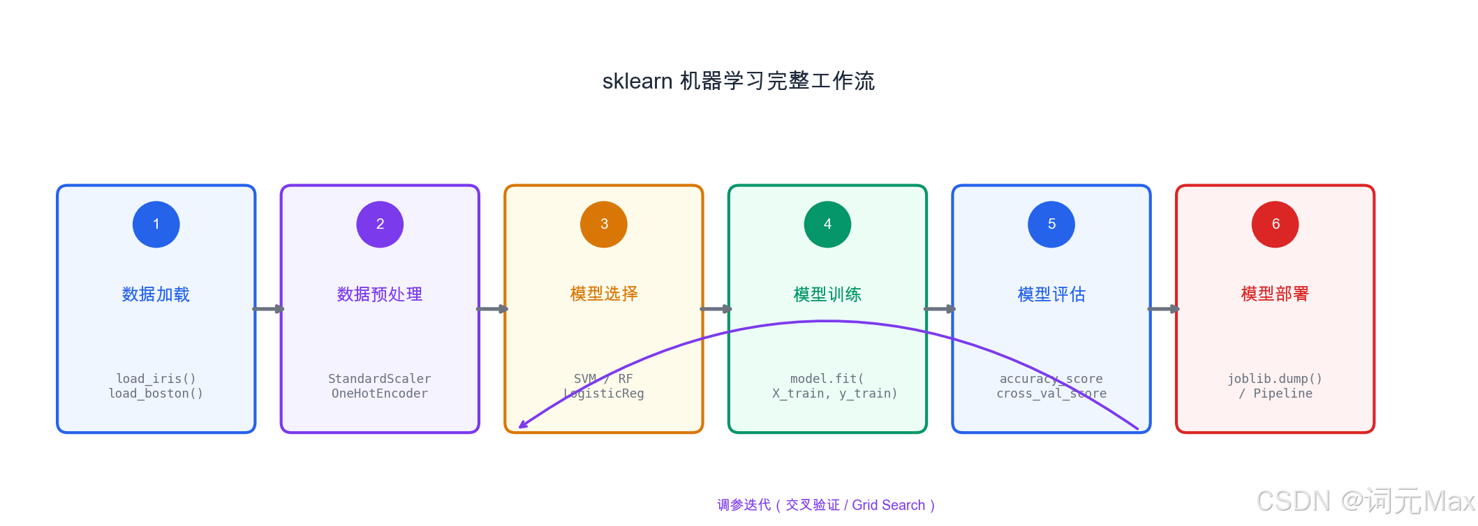
sklearn 机器学习完整工作流------从数据加载到模型部署的六个步骤

这是机器学习的"Hello World"，但我们做得比Hello World更完整：数据探索、多模型对比、混淆矩阵可视化、模型保存------这是真实项目的完整工作流。

1.1.1 这段代码在做什么

目标：在鸢尾花数据集（150个样本，4个特征，3个品种）上，比较4种分类算法的效果，选出最好的，保存模型并用它预测新样本。

1.1.2 步骤1：数据探索

在建模之前，先了解数据的基本情况：有多少样本、特征是什么、各类别分布是否均衡。

python 复制代码

import numpy as np
import pandas as pd
import matplotlib.pyplot as plt
import seaborn as sns
from sklearn.datasets import load_iris
from sklearn.model_selection import train_test_split, cross_val_score
from sklearn.preprocessing import StandardScaler
from sklearn.pipeline import Pipeline
from sklearn.ensemble import RandomForestClassifier, GradientBoostingClassifier
from sklearn.linear_model import LogisticRegression
from sklearn.svm import SVC
from sklearn.metrics import classification_report, confusion_matrix

# 加载数据
# iris.data: 形状(150, 4)，4个特征
# iris.target: 形状(150,)，0/1/2代表三个品种
iris = load_iris()
df = pd.DataFrame(iris.data, columns=iris.feature_names)
df['species'] = pd.Categorical.from_codes(iris.target, iris.target_names)

print("数据形状:", df.shape)          # (150, 5)
print("\n前5行:")
print(df.head())
print("\n统计信息:")
print(df.describe())
print("\n类别分布:")
print(df['species'].value_counts())   # 每种品种各50个，完全均衡

你应该看到：

数据集有150个样本、5列（4个特征+1个标签）
三种品种各50个，类别完全均衡
特征包括：花萼长度/宽度、花瓣长度/宽度

1.1.3 步骤2：多模型对比

这段代码在做什么：同时训练4种模型，用5折交叉验证比较它们的准确率，选出最好的。

python 复制代码

# 划分训练集和测试集
X = iris.data
y = iris.target

X_train, X_test, y_train, y_test = train_test_split(
    X, y, test_size=0.2, random_state=42,
    stratify=y  # 按类别比例分层抽样，保证训练/测试集中各类别比例一致
)

# 定义4种模型
# Pipeline：把数据预处理和模型训练串联成一个整体，防止数据泄露
models = {
    '逻辑回归': Pipeline([
        ('scaler', StandardScaler()),  # 标准化：统一特征的数值范围
        ('clf', LogisticRegression(max_iter=1000))
    ]),
    '随机森林': RandomForestClassifier(n_estimators=100, random_state=42),
    'SVM': Pipeline([
        ('scaler', StandardScaler()),
        ('clf', SVC(kernel='rbf', probability=True))
    ]),
    '梯度提升': GradientBoostingClassifier(n_estimators=100, random_state=42)
}

# 5折交叉验证比较所有模型
results = {}
print("5折交叉验证结果:")
for name, model in models.items():
    cv_scores = cross_val_score(model, X_train, y_train, cv=5)
    results[name] = cv_scores
    print(f"{name}: {cv_scores.mean():.4f} ± {cv_scores.std():.4f}")

你应该看到类似这样的输出：

复制代码

5折交叉验证结果:
逻辑回归: 0.9583 ± 0.0304
随机森林: 0.9583 ± 0.0304
SVM:     0.9750 ± 0.0190
梯度提升: 0.9500 ± 0.0354

所有模型准确率都在95%以上，说明这是个相对容易的数据集。SVM在这里表现最好。

1.1.4 步骤3：最佳模型评估

这段代码在做什么：用随机森林（通常最稳定）在测试集上做最终评估，并画出混淆矩阵。

python 复制代码

# 用随机森林做最终评估
best_model = models['随机森林']
best_model.fit(X_train, y_train)

y_pred = best_model.predict(X_test)
print("\n=== 最终评估（测试集）===")
print(classification_report(y_test, y_pred, target_names=iris.target_names))

# 混淆矩阵：行是真实类别，列是预测类别，对角线是预测正确的数量
cm = confusion_matrix(y_test, y_pred)
plt.figure(figsize=(8, 6))
sns.heatmap(cm, annot=True, fmt='d',
            xticklabels=iris.target_names,
            yticklabels=iris.target_names,
            cmap='Blues')
plt.title('混淆矩阵')
plt.ylabel('真实标签')
plt.xlabel('预测标签')
plt.show()

你应该看到：

精确率、召回率、F1分数都在95%以上
混淆矩阵的对角线值较大（预测正确的样本多），非对角线值很小（预测错误的样本少）

1.1.5 步骤4：保存和加载模型

这段代码在做什么：把训练好的模型保存到文件，然后加载回来预测一个新样本。

python 复制代码

import joblib

# 保存模型到文件
joblib.dump(best_model, 'iris_classifier.pkl')
print("模型已保存到 iris_classifier.pkl")

# 加载并预测一个新样本
loaded_model = joblib.load('iris_classifier.pkl')
sample = [[5.1, 3.5, 1.4, 0.2]]  # 一个新样本的4个特征
prediction = loaded_model.predict(sample)
prediction_proba = loaded_model.predict_proba(sample)

print(f"\n新样本特征: {sample[0]}")
print(f"预测品种: {iris.target_names[prediction[0]]}")  # 应该是 setosa
print(f"预测概率: {dict(zip(iris.target_names, prediction_proba[0].round(3)))}")

你应该看到：

复制代码

模型已保存到 iris_classifier.pkl
新样本特征: [5.1, 3.5, 1.4, 0.2]
预测品种: setosa
预测概率: {'setosa': 1.0, 'versicolor': 0.0, 'virginica': 0.0}

这个样本的花瓣很小（1.4和0.2），是setosa的典型特征，模型以100%的置信度预测正确。

1.2 项目2：房价预测（回归）

这个项目更贴近真实业务：处理缺失值、特征工程、多模型对比、误差分析。

1.2.1 这段代码在做什么

目标：在加州房价数据集上预测房价，比较线性模型和集成学习的效果，并分析哪些因素最影响房价。

1.2.2 步骤1：加载数据

python 复制代码

import numpy as np
import pandas as pd
from sklearn.datasets import fetch_california_housing
from sklearn.model_selection import train_test_split
from sklearn.preprocessing import StandardScaler
from sklearn.pipeline import Pipeline
from sklearn.ensemble import RandomForestRegressor, GradientBoostingRegressor
from sklearn.linear_model import LinearRegression, Ridge
from sklearn.metrics import mean_squared_error, r2_score, mean_absolute_error
import matplotlib.pyplot as plt

# 加载加州房价数据集
housing = fetch_california_housing()
df = pd.DataFrame(housing.data, columns=housing.feature_names)
df['MedHouseVal'] = housing.target  # 目标：房价（10万美元为单位）

print("数据形状:", df.shape)         # (20640, 9)
print("\n特征说明:")
feature_desc = {
    'MedInc': '收入中位数', 'HouseAge': '房屋年龄中位数',
    'AveRooms': '平均房间数', 'AveBedrms': '平均卧室数',
    'Population': '人口', 'AveOccup': '平均入住率',
    'Latitude': '纬度', 'Longitude': '经度'
}
for name, desc in feature_desc.items():
    print(f"  {name}: {desc}")

你应该看到：数据集有20640个样本，8个特征。收入中位数通常是预测房价最重要的特征。

1.2.3 步骤2：特征工程

从原始特征中构造更有意义的特征：

python 复制代码

# 特征工程：构造新特征
# 理由：rooms_per_household更有意义------平均每户有多少间房
df['rooms_per_household']  = df['AveRooms'] / df['AveOccup']
df['bedrooms_ratio']       = df['AveBedrms'] / df['AveRooms']      # 卧室比例
df['population_per_household'] = df['Population'] / df['AveOccup']  # 每户人口

feature_cols = housing.feature_names.tolist() + [
    'rooms_per_household', 'bedrooms_ratio', 'population_per_household'
]
X = df[feature_cols].values
y = df['MedHouseVal'].values

X_train, X_test, y_train, y_test = train_test_split(
    X, y, test_size=0.2, random_state=42
)

print(f"训练集: {X_train.shape[0]} 样本")
print(f"测试集: {X_test.shape[0]} 样本")
print(f"特征数: {X_train.shape[1]}")

你应该看到：训练集16512个样本，测试集4128个样本，11个特征（8个原始 + 3个新增）。

1.2.4 步骤3：模型训练与对比

这段代码在做什么：训练4种模型，比较它们在测试集上的RMSE（均方根误差）、MAE（平均绝对误差）和R²分数。

python 复制代码

# 定义4种模型
models = {
    '线性回归': Pipeline([
        ('scaler', StandardScaler()),
        ('reg', LinearRegression())
    ]),
    'Ridge回归': Pipeline([
        ('scaler', StandardScaler()),
        ('reg', Ridge(alpha=1.0))  # alpha：正则化强度，防止过拟合
    ]),
    '随机森林': RandomForestRegressor(
        n_estimators=100, random_state=42, n_jobs=-1
    ),
    '梯度提升': GradientBoostingRegressor(
        n_estimators=100, learning_rate=0.1, random_state=42
    )
}

print("模型对比（测试集）:")
print(f"{'模型':<15} {'RMSE':<12} {'MAE':<12} {'R²':<10}")
print("-" * 50)

for name, model in models.items():
    model.fit(X_train, y_train)
    y_pred = model.predict(X_test)

    # RMSE：均方根误差，单位和目标变量一致（10万美元）
    rmse = np.sqrt(mean_squared_error(y_test, y_pred))
    # MAE：平均绝对误差，更直观（平均误差多少10万美元）
    mae  = mean_absolute_error(y_test, y_pred)
    # R²：越接近1越好（模型解释了多少数据变化）
    r2   = r2_score(y_test, y_pred)

    print(f"{name:<15} {rmse:<12.4f} {mae:<12.4f} {r2:<10.4f}")

你应该看到类似这样的输出：

复制代码

模型对比（测试集）:
模型            RMSE         MAE          R²
--------------------------------------------------
线性回归        0.7268       0.5275       0.5758
Ridge回归       0.7268       0.5275       0.5759
随机森林        0.5079       0.3324       0.7783
梯度提升        0.4588       0.2995       0.8179

梯度提升的RMSE最小（约0.46，即平均误差约4.6万美元）、R²最高（0.82），说明它在这个数据集上效果最好。线性模型R²只有0.58，说明房价和特征之间不是简单的线性关系。

1.2.5 步骤4：误差分析

这段代码在做什么：可视化最佳模型的预测效果和误差分布，帮助理解模型在哪些区间预测得准、在哪些区间不准。

python 复制代码

# 使用最佳模型（梯度提升）做深入分析
best_model = models['梯度提升']
y_pred = best_model.predict(X_test)

# 预测值 vs 真实值：理想情况下所有点在对角线上
plt.figure(figsize=(10, 4))
plt.subplot(1, 2, 1)
plt.scatter(y_test, y_pred, alpha=0.3)
plt.plot([y_test.min(), y_test.max()],
         [y_test.min(), y_test.max()], 'r--', lw=2, label='理想预测')
plt.xlabel('真实房价（10万美元）')
plt.ylabel('预测房价（10万美元）')
plt.title('预测 vs 真实')
plt.legend()

# 残差分布：好的模型残差应接近正态分布且均值为0
plt.subplot(1, 2, 2)
residuals = y_test - y_pred
plt.hist(residuals, bins=50)
plt.xlabel('残差（真实值-预测值）')
plt.ylabel('频次')
plt.title('残差分布（越接近正态越好）')
plt.tight_layout()
plt.show()

print(f"\n残差统计:")
print(f"均值: {residuals.mean():.4f}（接近0说明模型无系统性偏差）")
print(f"标准差: {residuals.std():.4f}")

你应该看到：

预测 vs 真实图：大部分点分布在对角线附近，但高价房区域（>4的区域）预测偏差较大
残差分布：接近正态分布，均值接近0，说明模型无系统性偏差

1.3 Pipeline：工业级代码的标配

在实际项目中，数据往往有缺失值、混合类型特征等，Pipeline让你的代码更健壮、更不容易出错：

这段代码在做什么：展示如何用Pipeline处理同时含有数值和类别特征的真实数据，这是工业级ML代码的标准写法。

python 复制代码

from sklearn.pipeline import Pipeline
from sklearn.compose import ColumnTransformer
from sklearn.preprocessing import StandardScaler, OneHotEncoder
from sklearn.impute import SimpleImputer

# 真实场景：数据有缺失值、有数值和类别特征
numeric_features = ['age', 'income', 'score']
categorical_features = ['city', 'education']

# 数值特征处理：填充缺失值 + 标准化
numeric_transformer = Pipeline([
    ('imputer', SimpleImputer(strategy='median')),  # 用中位数填充缺失值
    ('scaler', StandardScaler())
])

# 类别特征处理：填充缺失值 + One-Hot编码
# One-Hot编码：把"北京/上海/广州"这样的类别变成0/1的数字表示
categorical_transformer = Pipeline([
    ('imputer', SimpleImputer(strategy='most_frequent')),
    ('encoder', OneHotEncoder(handle_unknown='ignore'))
])

# 组合处理器
preprocessor = ColumnTransformer([
    ('num', numeric_transformer, numeric_features),
    ('cat', categorical_transformer, categorical_features)
])

# 完整Pipeline：预处理 + 模型训练一体化
full_pipeline = Pipeline([
    ('preprocessor', preprocessor),
    ('classifier', RandomForestClassifier(n_estimators=100))
])

# 一行代码完成所有预处理和训练
# full_pipeline.fit(X_train, y_train)
# full_pipeline.predict(X_test)
print("Pipeline构建完成，调用 full_pipeline.fit() 即可开始训练")

Pipeline的三大好处：

防止数据泄露：StandardScaler的均值和方差只在训练集上计算，测试集用同样的参数变换，不会把测试集信息"泄露"进去
代码整洁：预处理和模型封装在一起，部署时只需保存一个Pipeline对象
方便调优：GridSearchCV可以直接在Pipeline上进行，搜索包括预处理参数在内的所有超参数

小结：sklearn完整工作流

复制代码

1. 数据探索（EDA）：了解数据形状、分布、缺失值
2. 特征工程：构造有意义的特征
3. 多模型对比：交叉验证，选最好的
4. 超参数调优：GridSearchCV或RandomizedSearchCV
5. 最终评估：在测试集上用正确的指标评估
6. 模型保存：joblib.dump

这个流程在实际工作中会反复使用。下一篇，我们看传统ML和LLM的分工------什么时候用哪个？