Bert理论讲解 - 技术栈

参考

B站尚硅谷，bert论文链接，李哥深度学习

概述

BERT（Bidirectional Encoder Representations from Transformers）是由 Google 于 2018 年提出的一种语言预训练模型。其核心创新在于采用 Transformer 的编码器（Encoder）结构，通过双向自注意力机制，在建模每个 token 表示时同时整合左右两个方向的上下文信息，从而获得更准确、更丰富的语义表示。

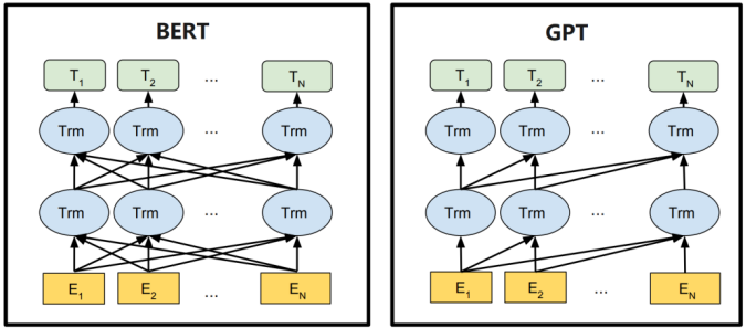
bert和g p t的区别在于是否能观察到全局信息还是只能观察到上文的信息

具体实现细节

预处理

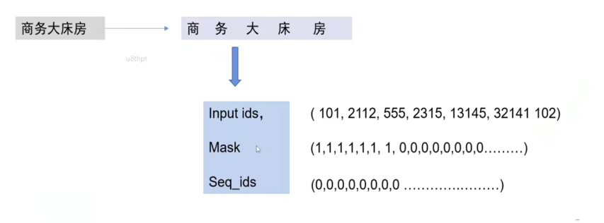
输入序号
掩码：我们输入的是固定长的句子但是掩码表示有效的句子长度
sequence ids用于分割句子

ids需要通过一个embedding

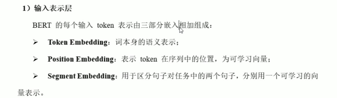
输入层表示，这个和tranfo,er不太一样，tranformer输入的有两个部分一个是embedding 一个是postional encoding 变成 token embedding

模型参数

本次实验做的是bert-base

模型版本	层数 (Layers)	模型维度 (d_model)	注意力头数 (Heads)	参数量
BERT-base	12	768	12	1.1 亿
BERT-large	24	1024	16	3.4 亿

Embedding类型	描述/作用	维度/形状	备注
Token Embedding	词元嵌入，表示输入序列中的每个token	(句子长度, 768)	768为模型隐藏层维度 (d_model)
Position Embedding	位置嵌入（最大限制）	(512, 768)	512为模型支持的最大输入长度
Segment Embedding	段嵌入，用于区分不同的句子片段（如NSP任务）	(2, 768)	2代表两句话

严谨起见（如果单纯了解可忽略）

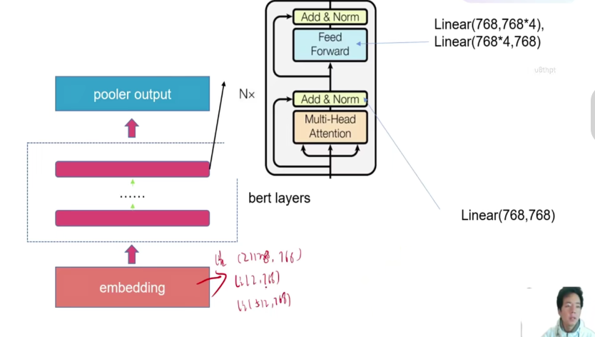
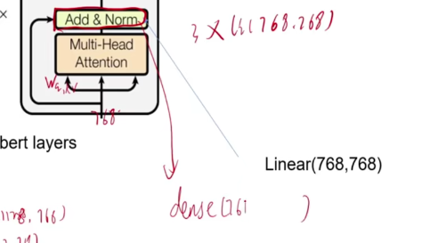
还需要经过dense层进一步提取

图片解析

左边的每一层都完全等同于右边的整个结构。

Dense层（全连接层）的核心作用是将前一层提取的特征进行整合与转化，最终输出任务所需的预测结果。它通过权重和偏置参数对输入特征进行线性变换，并结合非线性激活函数，增强模型的表达能力，使其能够拟合复杂的决策边界。

FFN层：升维度再降维

txt 复制代码

      [ 输入 x ]
      shape: (L, 768)
           |
           v
    +=========================================+
    |   >>> FEED FORWARD NETWORK (FFN) <<<    |
    |                                         |
    |    +-------------+                      |
    |    |  Linear 1   |  <-- 权重 W1: (768, 3072)
    |    |  (Dense)    |      把门打开，让信息量变大4倍
    |    +-------------+                      |
    |           |                             |
    |           v                             |
    |      shape: (L, 3072)  <-- 最宽处       |
    |           |                             |
    |      [ GELU/ReLU ]     <-- 激活函数      |
    |           |                             |
    |           v                             |
    |      shape: (L, 3072)                   |
    |           |                             |
    |           v                             |
    |    +-------------+                      |
    |    |  Linear 2   |  <-- 权重 W2: (3072, 768)
    |    |  (Dense)    |      把门关上，恢复原状
    |    +-------------+                      |
    |                                         |
    +=========================================+
           |
           v
      [ 输出 y ]
      shape: (L, 768)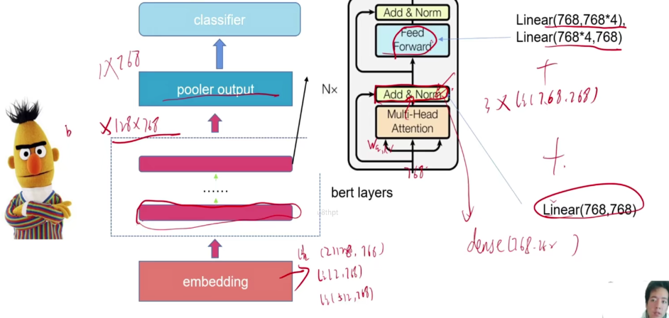

所以模型的参数分为3部分

直接运行理解参数

配置运行环境

sh 复制代码

conda create -n bert python=3.11 -y

conda activate bert

pip install torch==2.6.0 --index-url https://download.pytorch.org/whl/cpu

pip install transformers -i https://pypi.tuna.tsinghua.edu.cn/simple

前置知识

model.parameters() 返回一个生成器，生成参数

p.numl()

pytorch计算张量的方法

一个形状为 (768, 3072) 的权重矩阵，调用 .numel() 会返回 768 * 3072 = 2,359,296。
一个形状为 (768,) 的偏置向量，调用 .numel() 会返回 768。

bert的代码非常长，有时候能达到1000行，所以我们直接懂原理然后调用就可以

代码

py 复制代码

import os

# 设置 Hugging Face 镜像源，加速下载


from transformers import BertModel, BertTokenizer

# 1. 加载预训练模型（从 Hugging Face 镜像加载中文 BERT）
bert = BertModel.from_pretrained(r"E:\25.第二十五章 ⾃然语⾔处理通⽤框架-BERT实战\课件、源码\BERT开源项目及数据\bert-base-chinese")

# 2. 定义一个函数来统计模型参数
def get_parameter_number(model):
    # 计算总参数量 (Total Parameters)
    total_num = sum(p.numel() for p in model.parameters())
    
    # 计算可训练参数量 (Trainable Parameters)
    trainable_num = sum(p.numel() for p in model.parameters() if p.requires_grad)
    
    # 返回包含两个统计值的字典
    return {'Total': total_num, 'Trainable': trainable_num}

print(get_parameter_number(bert))
# 嵌入层三个输入 不用说了转换
emb_num = 21128*768 + 2*768 + 512*768  # 忽略了bias

# 参数说明 输入：每个词先通过嵌入层变成768维向量W_Q = 768×768 的矩阵  Query权重
#768 * 768 输出线性层
# 最后两个参数是前馈神经网络的升维和降维
self_att_num = 768*768*3 + 768*768 + 768*3072 + 3072*768
all_att_num = 12 * self_att_num  # 12层Transformer
pooler_num = 768*768#经过12层Transformer后，每个词都变成了768维向量
#取[CLS] token ：BERT会在句首添加一个特殊标记 [CLS]

print(emb_num + all_att_num + pooler_num)
# for name, para in bert.named_parameters():
#     print(name, para.shape)

结果和原理：我们的验证参数是对的

sh 复制代码

PS E:\25.第二十五章 ⾃然语⾔处理通⽤框架-BERT实战\课件、源码\BERT开源项目及数据> & D:/Software/Programming/Anaconda/envs/bert/python.exe "e:/25.第二十五章 ⾃然语⾔处理通⽤框架-BERT实战/课件、源码/BERT开源项目及数据/get_parm.py"
Loading weights: 100%|████████████████████████████████████████████████| 199/199 [00:00<00:00, 23911.83it/s]
[transformers] BertModel LOAD REPORT from: E:\25.第二十五章 ⾃然语⾔处理通⽤框架-BERT实战\课件、源码\BERT开 源项目及数据\bert-base-chinese
Key                                        | Status     |  | 
-------------------------------------------+------------+--+-
cls.seq_relationship.weight                | UNEXPECTED |  |
cls.predictions.bias                       | UNEXPECTED |  |
cls.predictions.transform.dense.weight     | UNEXPECTED |  |
cls.predictions.decoder.weight             | UNEXPECTED |  |
cls.predictions.transform.LayerNorm.bias   | UNEXPECTED |  |
cls.seq_relationship.bias                  | UNEXPECTED |  |
cls.predictions.transform.LayerNorm.weight | UNEXPECTED |  |
cls.predictions.transform.dense.bias       | UNEXPECTED |  |

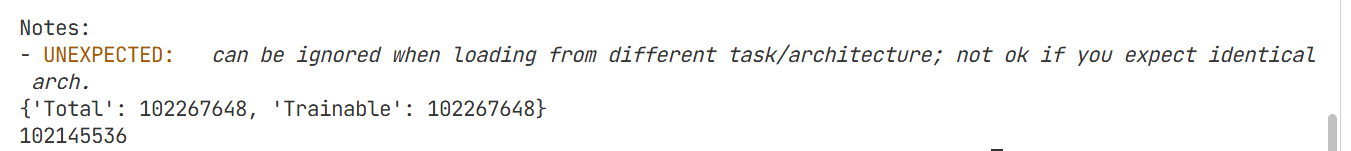
Notes:
- UNEXPECTED:   can be ignored when loading from different task/architecture; not ok if you expect identical arch.
{'Total': 102267648, 'Trainable': 102267648}
embeddings.word_embeddings.weight torch.Size([21128, 768])
embeddings.position_embeddings.weight torch.Size([512, 768])
embeddings.token_type_embeddings.weight torch.Size([2, 768])
embeddings.LayerNorm.weight torch.Size([768])
embeddings.LayerNorm.bias torch.Size([768])
encoder.layer.0.attention.self.query.weight torch.Size([768, 768])
encoder.layer.0.attention.self.query.bias torch.Size([768])
encoder.layer.0.attention.self.key.weight torch.Size([768, 768])
encoder.layer.0.attention.self.key.bias torch.Size([768])
encoder.layer.0.attention.self.value.weight torch.Size([768, 768])
encoder.layer.0.attention.self.value.bias torch.Size([768])
encoder.layer.0.attention.output.dense.weight torch.Size([768, 768])
encoder.layer.0.attention.output.dense.bias torch.Size([768])
encoder.layer.0.attention.output.LayerNorm.weight torch.Size([768])
encoder.layer.0.attention.output.LayerNorm.bias torch.Size([768])
encoder.layer.0.intermediate.dense.weight torch.Size([3072, 768])
encoder.layer.0.intermediate.dense.bias torch.Size([3072])
encoder.layer.0.output.dense.weight torch.Size([768, 3072])
encoder.layer.0.output.dense.bias torch.Size([768])
encoder.layer.0.output.LayerNorm.weight torch.Size([768])
encoder.layer.0.output.LayerNorm.bias torch.Size([768])
encoder.layer.1.attention.self.query.weight torch.Size([768, 768])
encoder.layer.1.attention.self.query.bias torch.Size([768])
encoder.layer.1.attention.self.key.weight torch.Size([768, 768])
encoder.layer.1.attention.self.key.bias torch.Size([768])
encoder.layer.1.attention.self.value.weight torch.Size([768, 768])
encoder.layer.1.attention.self.value.bias torch.Size([768])
encoder.layer.1.attention.output.dense.weight torch.Size([768, 768])
encoder.layer.1.attention.output.dense.bias torch.Size([768])
encoder.layer.1.attention.output.LayerNorm.weight torch.Size([768])
encoder.layer.1.attention.output.LayerNorm.bias torch.Size([768])
encoder.layer.1.intermediate.dense.weight torch.Size([3072, 768])
encoder.layer.1.intermediate.dense.bias torch.Size([3072])
encoder.layer.1.output.dense.weight torch.Size([768, 3072])
encoder.layer.1.output.dense.bias torch.Size([768])
encoder.layer.1.output.LayerNorm.weight torch.Size([768])
encoder.layer.1.output.LayerNorm.bias torch.Size([768])
encoder.layer.2.attention.self.query.weight torch.Size([768, 768])
encoder.layer.2.attention.self.query.bias torch.Size([768])
encoder.layer.2.attention.self.key.weight torch.Size([768, 768])
encoder.layer.2.attention.self.key.bias torch.Size([768])
encoder.layer.2.attention.self.value.weight torch.Size([768, 768])
encoder.layer.2.attention.self.value.bias torch.Size([768])
encoder.layer.2.attention.output.dense.weight torch.Size([768, 768])
encoder.layer.2.attention.output.dense.bias torch.Size([768])
encoder.layer.2.attention.output.LayerNorm.weight torch.Size([768])
encoder.layer.2.attention.output.LayerNorm.bias torch.Size([768])
encoder.layer.2.intermediate.dense.weight torch.Size([3072, 768])
encoder.layer.2.intermediate.dense.bias torch.Size([3072])
encoder.layer.2.output.dense.weight torch.Size([768, 3072])
encoder.layer.2.output.dense.bias torch.Size([768])
encoder.layer.2.output.LayerNorm.weight torch.Size([768])
encoder.layer.2.output.LayerNorm.bias torch.Size([768])
encoder.layer.3.attention.self.query.weight torch.Size([768, 768])
encoder.layer.3.attention.self.query.bias torch.Size([768])
encoder.layer.3.attention.self.key.weight torch.Size([768, 768])
encoder.layer.3.attention.self.key.bias torch.Size([768])
encoder.layer.3.attention.self.value.weight torch.Size([768, 768])
encoder.layer.3.attention.self.value.bias torch.Size([768])
encoder.layer.3.attention.output.dense.weight torch.Size([768, 768])
encoder.layer.3.attention.output.dense.bias torch.Size([768])
encoder.layer.3.attention.output.LayerNorm.weight torch.Size([768])
encoder.layer.3.attention.output.LayerNorm.bias torch.Size([768])
encoder.layer.3.intermediate.dense.weight torch.Size([3072, 768])
encoder.layer.3.intermediate.dense.bias torch.Size([3072])
encoder.layer.3.output.dense.weight torch.Size([768, 3072])
encoder.layer.3.output.dense.bias torch.Size([768])
encoder.layer.3.output.LayerNorm.weight torch.Size([768])
encoder.layer.3.output.LayerNorm.bias torch.Size([768])
encoder.layer.4.attention.self.query.weight torch.Size([768, 768])
encoder.layer.4.attention.self.query.bias torch.Size([768])
encoder.layer.4.attention.self.key.weight torch.Size([768, 768])
encoder.layer.4.attention.self.key.bias torch.Size([768])
encoder.layer.4.attention.self.value.weight torch.Size([768, 768])
encoder.layer.4.attention.self.value.bias torch.Size([768])
encoder.layer.4.attention.output.dense.weight torch.Size([768, 768])
encoder.layer.4.attention.output.dense.bias torch.

流程

我主要挑1些对我自己来说需要强调的就行其他的自己了解

输入和embedding

假设输入一句话：["我", "爱", "中国"]

第一步 ：每个词先通过嵌入层变成768维向量

复制代码

"我"   → [0.1, 0.2, ..., 0.9]  (768维)
"爱"   → [0.3, 0.5, ..., 0.1]  (768维)
"中国" → [0.7, 0.2, ..., 0.4]  (768维)

自注意力QKV运算

bert也是利用到自注意力计算的

第二步 ：用三个权重矩阵分别计算 Q、K、V

python 复制代码

W_Q = 768×768 的矩阵  # Query权重
W_K = 768×768 的矩阵  # Key权重  
W_V = 768×768 的矩阵  # Value权重

Q = 输入 × W_Q  # 每个词的Query向量
K = 输入 × W_K  # 每个词的Key向量
V = 输入 × W_V  # 每个词的Value向量

**pooler_num = 768×768 的含义**

这是 池化层（Pooler） 的参数，用来把整个句子的表示"浓缩"成一个固定向量。

池化层

复制代码

输入："我 爱 中 国"
       ↓
   BERT编码器
       ↓
输出：每个词都有一个768维向量
       ↓
   池化层
       ↓
输出：一个768维的句子向量  ← 用于分类等任务

输入：经过12层Transformer后，每个词都变成了768维向量
复制代码
```
"我"   → [768维]
"爱"   → [768维]
"中国" → [768维]
```
取 $CLS$ token ：BERT会在句首添加一个特殊标记 [CLS]
复制代码
```
[[CLS], 我, 爱, 中, 国]
     ↑
取这个位置的向量
```

全连接层处理：

python 复制代码

# 池化层：768 → 768 的线性变换
句子向量 = 全连接层([CLS]的768维向量)

# 参数 = 768 × 768

为什么叫"池化"？

"池化"（Pooling）来源于 CNN 的概念，但这里的 BERT Pooler 其实是：

python 复制代码

class Pooler(nn.Linear):
    def __init__(self):
        super().__init__(768, 768)  # 768×768

它本质是一个全连接层，不是真正的池化（如Max Pooling）。但习惯上叫它"池化层"。