PyTorch计算机视觉(4)------迁移学习(Transfer Learning)详解与实现
0. 前言
在计算机视觉项目中设计合适的卷积神经网络 (Convolutional Neural Network, CNN)模型并非易事,ResNet9 模型架构是针对低分辨率图像数据集最简洁高效的模型之一。对于高分辨率图像数据集,则需要采用更强大的模型。现有许多基于数百万张图像训练得到的优秀预训练模型可供利用,因此我们无需重复造轮子。迁移学习 (Transfer Learning) 正是运用这些预训练模型处理新数据集的图像分类或其他计算机视觉任务的有效方法。
1. 迁移学习基本概念
迁移学习 (Transfer Learning) 指利用已经学习好的模型在新任务上具有良好的表现和推广能力的机器学习技术,能够将通用数据集上的模型学习迁移到特定数据集中。通常,用于执行迁移学习的预训练模型在数百万张图像(通用大型数据集)上进行训练,然后使用特定感兴趣数据集微调预训练模型。

2. 迁移学习的重要性
假设我们需要处理道路图像,并根据图像包含的对象进行分类,而从零开始构建、训练模型可能会因为图像的数量不足,而难以学习到数据集中的各种变化,对 8,000 张图像进行训练比在 2000 张图像上进行训练的模型准确率更高。在 ImageNet 上训练的预训练模型能够很好的解决该问题,在对 ImageNet 数据集进行训练期间,模型已经学习了很多与交通相关的特征,例如汽车、道路、树木和人等。因为模型已经学习了大量通用特征,因此,利用已经训练好的模型能够更快和更准确的训练新模型,只需要将预训练模型提取到的特征用于新模型的训练,就可以得到适用于目标任务的性能优异的新模型。
3. ImageNet
ImageNet 是一个大规模图像数据集,该数据集包含了超过 1400 万张标注图像,覆盖了 1 万多个分类标签。ImageNet 数据集被广泛用于计算机视觉领域中,包括自动驾驶、智能监控、医学影像分析等。ImageNet 挑战赛由 ImageNet 项目组于 2010 年开始举办,是计算机视觉领域的顶尖比赛之一。在本节中,将使用在 ImageNet 数据集上预训练的深度神经网络构建迁移学习模型。
4. 迁移学习流程
迁移学习的一般流程如下:
- 归一化输入图像,使用与预训练模型训练期间相同的均值和标准差进行归一化
- 获取在大型数据集上进行预训练模型的架构与模型权重
- 丢弃预训练模型的最后几层
- 将截断的预训练模型连接到一个或多个新初始化的神经网络层,并确保最后一层的神经元与需要预测的类别数(输出)相同
- 确保预训练模型的权重不可更新(即在反向传播期间冻结预训练模型参数),但新初始化的神经网络层权重是可训练的。因为预训练模型权重已经使用大型数据集进行了很好的训练,因此可以利用从大型模型中学习到的特征而无需对预训练模型进行训练,而只需要利用小数据集训练新初始化的神经网络层
- 更新可训练参数,拟合模型
我们已经了解了如何实现迁移学习,接下来,我们介绍预训练卷积神经网络架构 ResNet,并使用迁移学习将预训练模型应用于蔬菜图像分类任务。
5. 使用 ResNet 进行迁移学习
运行以下代码,可以看到超过百种预训练模型,包括 resnet18、resnet34、resnet50、resnet101、resnet152 以及 vgg16 等。这些预训练模型原本针对 224×224 尺寸图像设计,本节将改造并使用 resnet18、resnet50 和 resnet152 模型进行蔬菜图像分类。
python
import torchvision
import torchvision.models
dir(models)
蔬菜图像分类项目包含三个部分:第一部分负责导入数据集、构建数据加载器并展示样本图像及其标签。从 Kaggle 下载的 zip 文件大小约为 560MB,解压至 VegetableImgs 文件夹后可见三个子文件夹 train、test 和 validation,每个文件夹下包含 15 个以蔬菜种类命名的二级子文件夹。通过使用 torchvision 的 ImageFolder 工具将这些图像打包成三个数据集,运行 train_dataset.classes 可以看到这 15 个类别的名称列表:Bean(豆类)、Bitter_Gourd(苦瓜)、Bottle_Gourd(瓶瓜)、Brinjal(茄子)、Broccoli(西兰花)、Cabbage(卷心菜)、Capsicum(辣椒)、Carrot(胡萝卜)、Cauliflower(花椰菜)、Cucumber(黄瓜)、Papaya(木瓜)、Potato(土豆)、Pumpkin(南瓜)、Radish(萝卜)和Tomato(西红柿)。由于原始图像尺寸不一致,且多数为 224×224 分辨率,为节省训练时间我们将统一调整为 128×128 分辨率。
python
import torch; import torch.nn as nn; from torch.utils.data import DataLoader
import torch.optim.lr_scheduler as lr_scheduler
from torchvision.utils import make_grid; from torchvision import models
from torchvision.datasets import ImageFolder
from torchvision import transforms as T;
from matplotlib import pyplot as plt
import numpy as np; import pandas as pd; from tqdm import tqdm, trange
n_epochs = 10
img_size = (224, 224); img_channels = 3
batch_size=64
lr =1e-2
data_path = './VegetableImgs/'
将三个数据集分别载入批大小为 64 的数据加载器,下图展示了训练图像的数据样本,其中部分图像因 RandomVerticalFlip 增强处理呈现倒置效果。第二部分包含预训练模型、损失函数、优化器及学习率调度器的配置。最后部分则用于模型训练及结果可视化。
python
train_dataset = ImageFolder(root=data_path+'train/', transform=T.Compose([
                        T.Resize(img_size),
                        T.RandomVerticalFlip(0.5),
                        T.RandomHorizontalFlip(p=0.5),
                        T.ToTensor(),
                        T.Normalize([0.5,0.5,0.5], [0.5,0.5,0.5])]))
val_dataset = ImageFolder(root=data_path+'validation/', transform=T.Compose([
                        T.Resize(img_size),
                        T.ToTensor(),
                        T.Normalize([0.5,0.5,0.5], [0.5,0.5,0.5])]))
test_dataset = ImageFolder(root=data_path+'test/', transform=T.Compose([
                        T.Resize(img_size),
                        T.ToTensor(),
                        T.Normalize([0.5,0.5,0.5], [0.5,0.5,0.5])]))
classes = train_dataset.classes; n_class = len(classes)
s_p_e = int(len(train_dataset)/batch_size); n_samples=s_p_e * batch_size
train_dataloader = DataLoader(train_dataset, batch_size=batch_size, shuffle=True,
                    num_workers=4, pin_memory=True, drop_last=True)
val_dataloader = DataLoader(val_dataset, batch_size=batch_size, shuffle=False,
                    num_workers=4, pin_memory=True, drop_last=True)
test_dataloader = DataLoader(test_dataset, batch_size=batch_size, shuffle=False,
                    num_workers=4, pin_memory=True, drop_last=True)
n_batch = len(train_dataloader)
for imgs, labels in train_dataloader:
    print(imgs.shape, '\nlables=', labels); break
def denorm(img_tensors): # Shift image pixel values to [0,1]
    return img_tensors * 0.5 + 0.5
def show_imgs(images):
    fig, ax = plt.subplots(figsize=(16,10))
    inputs = make_grid(denorm(images[:16]), nrow=8)
    ax.imshow(inputs.permute(1,2,0))
    ax.set(xticks=[], yticks=[])
show_imgs(imgs)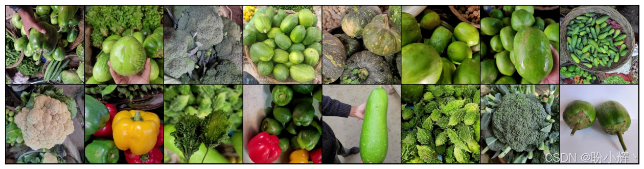
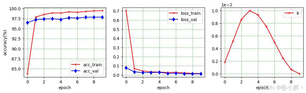
默认情况下,torchvision 提供的所有预训练模型都适用于包含 1000 个类别的图像数据集。如果执行 print(model),会发现 resnet18 模型的最后一层是一个全连接层:nn.Linear(1024, 1000, bias=False)。该层原本为包含 1000 个类别的 ImageNet 数据集设计,因此我们需要针对仅含 15 个类别的蔬菜图像数据集修改最后一层参数。修改完成后运行 print(model),会看到最终的全连接层已变为 nn.Linear(1024,15, bias=False)。我们还可以通过 pretrained=True 选项导入优化后的预训练模型参数。尝试 False 选项,会发现分类准确度较低。如果一些代码前的 # 符号,代码将冻结预训练模型中的所有参数。由于最后一层全连接层已被修改,此时仅最后一层的参数会在模型训练过程中更新。但这种情况下的分类准确率并不理想。更新所有预训练的 resnet18 模型的参数时,测试数据加载器的分类准确率可达约 98%,如下图所示。若使用 resnet50 和 resnet101 模型,准确率会有小幅提升,但训练时间将分别延长至两倍和三倍。
python
model = models.resnet18(pretrained=True)
print(model)
model.eval()
for param in model.parameters():
    param.requires_grad = False
num_ftrs = model.fc.in_features
model.fc = nn.Linear(num_ftrs, n_class)
model = model.cuda()
criterion = nn.CrossEntropyLoss(reduction='sum')
optimizer = torch.optim.SGD(model.parameters(), lr=lr)
scheduler = lr_scheduler.OneCycleLR(optimizer, max_lr=lr,
        steps_per_epoch=s_p_e, epochs=n_epochs, pct_start=0.4)
def training(my_dataloader):
    total_loss = 0.0; n_correct = 0.0
    n_samples = len(my_dataloader.dataset)
    model.train()
    for images, labels in my_dataloader:
        labels = labels.cuda(non_blocking=True)
        outputs = model(images.cuda(non_blocking=True))
        predictions = torch.argmax(outputs, dim=1)
        n_correct += torch.sum(predictions==labels).item()
        loss = criterion(outputs, labels)
        total_loss += loss.item()
        loss.backward()
        nn.utils.clip_grad_value_(model.parameters(), clip_value=0.1)
        optimizer.step()
        scheduler.step()
        optimizer.zero_grad()
    return total_loss/n_samples, 100*n_correct/n_samples
def evaluation(my_dataloader):
    n_samples = len(my_dataloader.dataset)
    with torch.no_grad():
        total_loss = 0.0; n_correct = 0
        model.eval()
        for images, labels in my_dataloader:
            labels = labels.cuda(non_blocking=True)
            outputs = model(images.cuda(non_blocking=True))
            predictions = torch.argmax(outputs, dim=1)
            n_correct += torch.sum(predictions==labels).item()
            loss = criterion(outputs, labels)
            total_loss += loss.item()
    return total_loss/n_samples, 100*n_correct/n_samples
def fitting(epochs):
    df = pd.DataFrame(np.empty([epochs, 5]),
        index = np.arange(epochs),
        columns=['loss_train', 'acc_train', 'loss_val', 'acc_val', 'lr'])
    progress_bar = trange(epochs)
    for i in progress_bar:
        df.iloc[i,0], df.iloc[i,1] = training(train_dataloader)
        df.iloc[i,2], df.iloc[i,3] = evaluation(val_dataloader)
        df.iloc[i,4] = optimizer.param_groups[0]['lr']
        progress_bar.set_description("train_loss=%.5f" % df.iloc[i,0])
        progress_bar.set_postfix(
                    {'train_acc': df.iloc[i,1], 'val_acc': df.iloc[i,3]})
    return df
train_history = fitting(n_epochs)
df= train_history
fig, ax = plt.subplots(1,3, figsize=(12,3), sharex=True)
df.plot(ax=ax[0], y=[1,3], style=['r-+', 'b-d'])
df.plot(ax=ax[1], y=[0,2], style=['r-+', 'b-d'])
df.plot(ax=ax[2], y=[4], style=['r-+'])
for i in range(3):
    ax[i].set_xlabel('epoch')
    ax[i].grid(which='major', axis='both', color='g', linestyle=':')
ax[0].set_ylabel('accuracy(%)')
ax[2].ticklabel_format(style='sci', axis='y', scilimits=(0,0))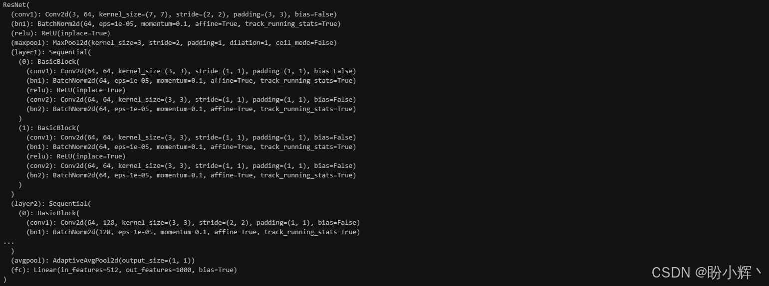
对测试数据集中指定索引的单个图像进行分类,并输出该图像以供验证分类结果。
python
loss, accuracy = evaluation(test_dataloader)
print('test dataloader accuracy (%)=', accuracy)
n = 1300
img, label = test_dataset[n]
def predict_image(img, model):
    print('img.shape=', img.shape)
    x = img.unsqueeze(0).cuda()
    print('img.unsqueeze(0).shape=', x.shape)
    y = model(x)
    preds = torch.argmax(y, dim=1)
    return train_dataset.classes[preds[0].item()]
print('Prediction is: {0}; Label is {1}'.format(
        predict_image(img, model), train_dataset.classes[label]))
plt.imshow(denorm(img).permute(1,2,0))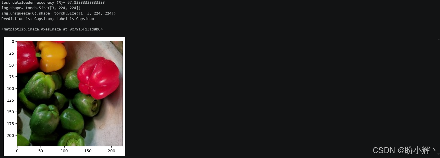
通过以下 ResNet18 模型的结构解析,将理解预训练 ResNet 模型内部包含哪些代码。其中名为 basic 的函数包含两个卷积层,该函数的输入为 4D 张量,输出同样为 4D 张量,但其通道数和分辨率可能与输入不同。
python
# Simple ResNet18 ---------------------------------------------------------------
import torch.nn as nn; from torchsummary import summary
def basic(in_channels, out_channels, stride=1):
    return nn.Sequential(nn.Conv2d(in_channels, out_channels, kernel_size=3,
                                stride=stride, padding=1, bias=False),
                        nn.BatchNorm2d(out_channels),
                        nn.ReLU(inplace=True),
                        nn.Conv2d(out_channels, out_channels, kernel_size=3,
                                stride=1, padding=1, bias=False),
                        nn.BatchNorm2d(out_channels))
class Id_Block(nn.Module):
    def __init__(self, in_channels, out_channels, stride=1):
        super().__init__()
        self.basic_block = basic(in_channels, out_channels, stride=stride)
        self.relu = nn.ReLU()
    def forward(self, x):
        return self.relu(x + self.basic_block(x))
class Rs_Block(nn.Module):
    def __init__(self, in_channels, out_channels, stride=2):
        super().__init__()
        self.basic_block = basic(in_channels, out_channels, stride=2)
        self.shortcut = nn.Sequential(
                nn.Conv2d(in_channels, out_channels, kernel_size=1,
                            stride=stride, padding=0, bias=False),
                            nn.BatchNorm2d(out_channels))
        self.relu = nn.ReLU()
    def forward(self, x):
        return self.relu(self.shortcut(x) + self.basic_block(x))
class ResNet(nn.Module):
    def __init__(self, image_channels=3, num_classes=10):
        super().__init__()
        self.net = nn.Sequential(
                        nn.Conv2d(in_channels=image_channels, out_channels=64,
                            kernel_size=7, stride=2, padding=3, bias=False),
                        nn.BatchNorm2d(64),
                        nn.ReLU(),          # shape = -1 x 64 x 112 x 112
                        nn.MaxPool2d(kernel_size=3, stride=2, padding=1),
                        Id_Block(64, 64, 1), Id_Block(64, 64, 1),
                        Rs_Block(64, 128, 2), Id_Block(128, 128, 1),
                        Rs_Block(128, 256, 2), Id_Block(256, 256, 1),
                        Rs_Block(256, 512, 2), Id_Block(512, 512, 1),
                        nn.AdaptiveAvgPool2d(1),    # shape = -1 x 64 x 1 x 1
                        nn.Flatten(),
                        nn.Linear(512, num_classes)
                        )
    def forward(self, imgs):    #imgs.shape = -1 x 3 x 224 x 224
        return self.net(imgs)   #ioutput.shape = -1 x n_classes
model = ResNet().cuda()
summary(model, (3,224,224))     #print details of the model Params: 42.65MB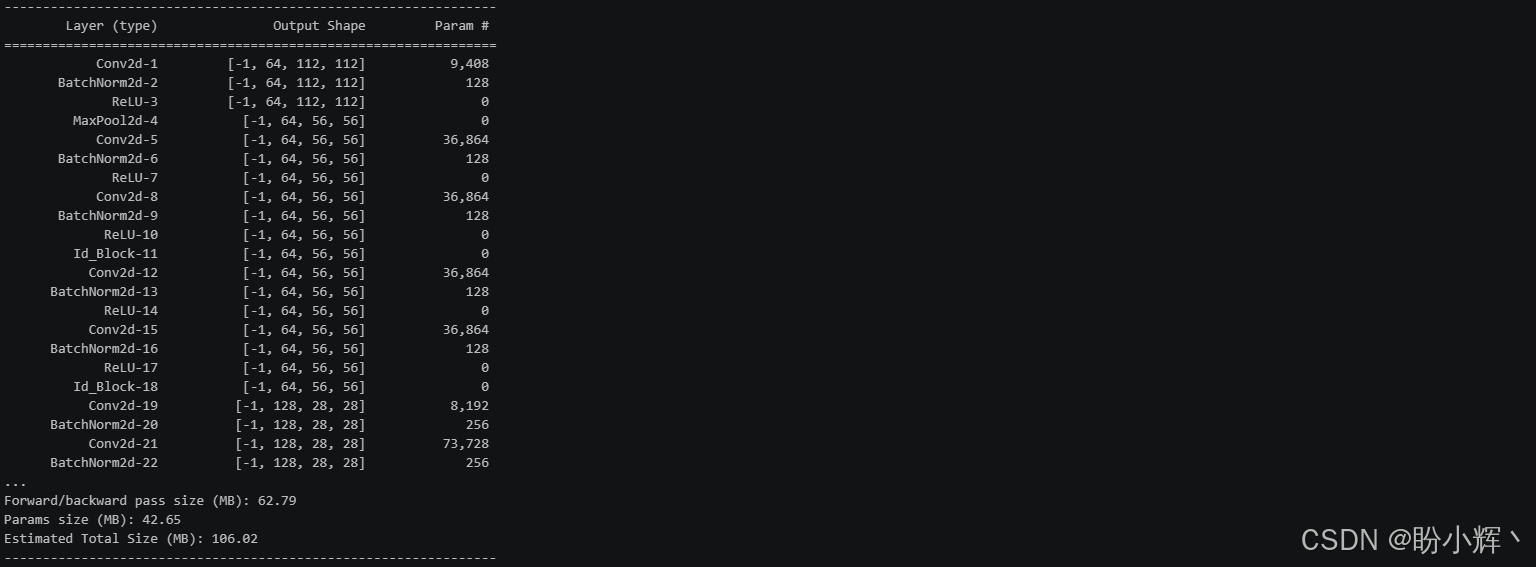
定义名为 Id_Block 的类包含两个分支:其基础分支的输入与输出保持相同维度;另一分支则直接输出输入张量本身。两个分支的输出会直接相加作为该类的最终输出。而命名为 Rs_Block 的类同样具有双分支结构:与输入张量维度相比,其基础分支(步长=2)输出的通道数和分辨率会发生改变;另一个名为 shortcut 的分支通过核大小为 1 的卷积层对输入张量进行变换,从而使第二分支的输出维度能与基础分支输出维度匹配。这些基础模块共同构成了 ResNet18 模型的完整架构。
ResNet18 模型包含 17 个卷积层和 1 个全连接层,这正是其命名为 ResNet18 的原因。运行代码 p_list = [p.numel() for p in model.parameters()]; print(sum(p_list),' = ', p_list),将得到 resnet18 模型参数总量( 11181642 个)及各层参数数量分布。若切换至其他预训练模型并查看参数数量,会发现 resnet50 模型的参数总量达到 23528522 个。通过运行以下代码,我们可以打印出所有参数名称及其维度:输出的首行可见名为 conv1.weight 的参数,其维度为 torch.Size([64, 3, 7, 7]),这就是 ResNet18 模型第一个卷积层中卷积操作的权重张量。
python
for name, parameter in model.named_parameters():
    print(name, '\t\t', parameter.shape)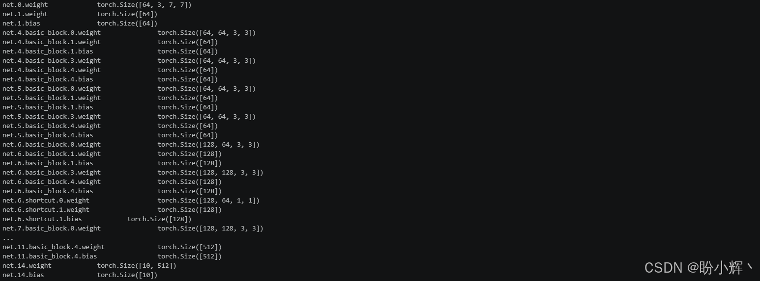
该卷积权重张量可视为包含 64 个样本、3 个通道、分辨率为 7×7 的图像批次。通过后续代码可可视化这批图像,此时权重张量的每个元素值都被归一化至 [0,1] 区间。下图可视化了来自经过参数优化的预训练 ResNet18 模型,可以看到层数更深的 ResNet 模型能够提取图像更精细的特征模式信息。
python
fig, ax = plt.subplots(figsize=(7, 7))
w = model.conv1.weight.cpu()
min_w=torch.min(w)
w1 = (-1/(2*min_w))*w + 0.5
img_grid = make_grid(w1, nrow=8, padding=1)
ax.imshow(img_grid.permute(1,2,0))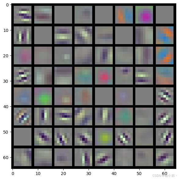
小结
本节介绍了迁移学习的概念、重要性及实现流程,并基于 ResNet 预训练模型完成了蔬菜图像分类任务。迁移学习通过利用在 ImageNet 等大型数据集上预训练的模型权重,有效解决了小样本数据集训练困难的问题。实验表明,微调 resnet18 模型在测试集上可达约 98% 的分类准确率。最后通过可视化模型参数,展示了预训练模型各层提取的特征模式,加深了对深度网络内部机制的理解。
系列链接
PyTorch计算机视觉(1)------计算机视觉的数学工具