2025年五一杯数学建模
A题 支路车流量推测问题
原题再现:
在道路网络中,主路通常配备车流量监测设备,能够实时记录主路的车流量数据。当多条支路汇入主路时,由于部分支路未安装车流量监测设备,各支路的车流量需要结合主路的车流量数据和支路车流量的历史趋势信息进行推测。这将为优化交通信号灯的配时、缓解交通拥堵和规划道路资源等问题提供数据和方法支持。
本题目中假设:(1) 主路上的车流量是各支路车流量的总和,且各支路的车流量具有一定的规律性 (如早晚高峰、平峰时段的车流量分布不同),这种规律性可以用函数来描述;(2) 道路均为单向车道,图 1‑图 3 中的蓝色箭头代表车流方向;(3) 问题 1‑问题 4 中车流量的 "增长 / 减少" 趋势均指 "严格单调增长 / 严格单调减少" 趋势,"稳定" 指车流量稳定为某固定非负常数,各支路流量变化的函数关系均为连续函数;(4) 车流量记录数据已换算为标准车当量数,各问题中的车流量均指标准车当量数,可为任意非负实数,不考虑车流量单位。
请依据附件,建立数学模型,完成以下问题。
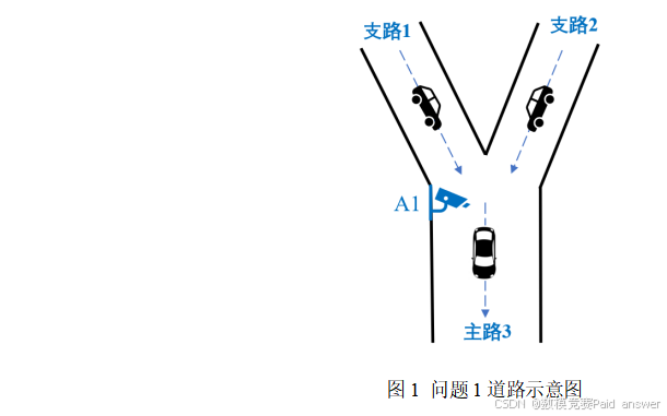
问题 1. 考虑图 1 所示的 Y 型道路,支路 1 和支路 2 的车流同时汇入主路 3。假设仅在主路 3 上安装了车流量监测设备 A1,每 2 分钟记录一次主路的车流量信息,车辆从支路汇入主路后行驶到 A1 处的时间忽略不计。附件表 1 中提供了某天早上 6:58,8:58 主路 3 上的车流量数据 (7:00 为第一个数据记录时刻,8:58 是最后一个数据记录时刻,下同)。
由历史车流量观测记录可知,在 6:58,8:58 时间段内,支路 1 的车流量呈现线性增长趋势,支路 2 的车流量呈现先线性增长后线性减少的趋势。
请建立数学模型,根据附件表 1 的数据推测在 6:58,8:58 时间段内支路 1 和支路 2 上的车流量,并使用合适的函数关系来描述支路 1、支路 2 的车流量随时间 t 的变化 (为方便起见,函数关系中令 7:00 为 t=0,t 属于 0,59,下同),在表 1.1 中填入具体的函数表达式。

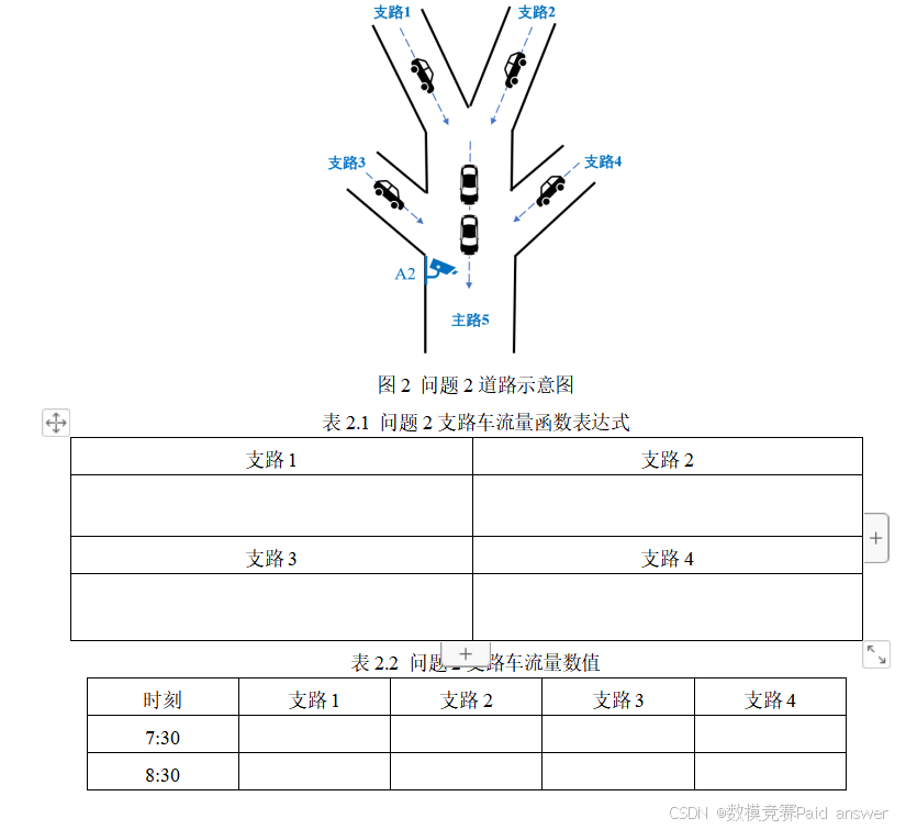
问题 2. 考虑图 2 所示的道路,支路 1 和支路 2 的车流同时汇入主路 5,支路 3 和支路 4 的车流同时汇入主路 5,仅在主路 5 上安装了车流量监测设备 A2,每 2 分钟记录一次主路的车流量信息,附件表 2 中提供了某天早上 6:58,8:58 时间段内主路 5 上的车流量数据。假设车辆从支路 1 和支路 2 的路口行驶到设备 A2 处的时间为 2 分钟,车辆从支路 3 和支路 4 的路口到达设备 A2 处的行驶时间忽略不计。
由历史车流量观测记录可知,在 6:58,8:58 时间段内,支路 1 的车流量稳定;支路 2 的车流量在 6:58,7:48 和 8:14,8:58 时间段内线性增长,在 (7:48,8:14) 时间段内稳定;支路 3 的车流量呈现先线性增长后稳定的趋势;支路 4 的车流量呈现周期性规律。
请建立数学模型,根据附件表 2 的数据推测支路 1、支路 2、支路 3、支路 4 上的车流量,使用合适的函数关系来描述各支路上的车流量随时间的变化,并分析结果的误差。在表 2.1 中填入具体的函数表达式,在表 2.2 中分别填入 7:30 和 8:30 这两个时刻各支路上的车流量数值。
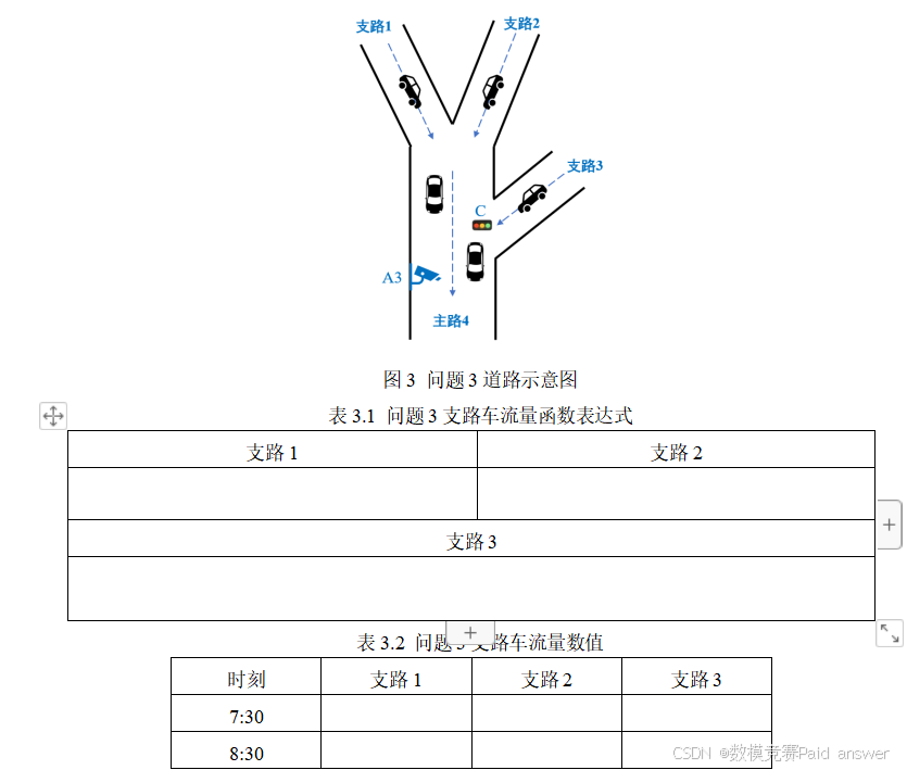
问题 3. 考虑图 3 所示的道路,支路 1、支路 2 的车流同时汇入主路 4,支路 3 为特殊交通管制路段,支路 3 上的车辆通过路口时受到交通信号灯 C 的控制。C 的红灯时间设置为 8 分钟,绿灯时间设置为 10 分钟,黄灯时间忽略不计。仅在主路 4 上安装了车流量监测设备 A3,每 2 分钟记录一次主路的车流量信息,附件表 3 中提供了某天早上 6:58,8:58 主路 4 上的车流量数据。假设车辆从支路 1 和支路 2 的路口处到达 A3 处的行驶时间为 2 分钟,车辆从支路 3 汇入主路后到达设备 A3 处的行驶时间忽略不计。
由历史车流量观测记录可知,在 6:58,8:58 时间段内,支路 1 的车流量呈现 "无车流量→增长→减少→稳定→减少至无车流量" 的趋势;支路 2 的车流量分别在 6:58,8:10 和 8:34,8:58 时间段内线性增长和线性减少,在 (8:10,8:34) 时间段内稳定。当 C 显示绿灯时,支路 3 的车流量或稳定或呈现线性变化趋势,且第一个绿灯于 7:06 时开始亮起;当 C 显示红灯时,支路 3 的车流量视为 0。
请建立数学模型,根据附件表 3 的数据推测支路 1、支路 2、支路 3 上的车流量,使用合适的函数关系来描述各支路上的车流量随时间的变化,并分析结果的误差。在表 3.1 中填入具体的函数表达式,在表 3.2 中分别填入 7:30 和 8:30 这两个时刻各支路上的车流量数值。
问题 4. 在网络信号弱、能见度低、车流量较大或车速过快等情况下,车流量监测设备可能会产生数据误差。考虑图 3 所示的道路,假设某天设备 A3 记录的数据产生了误差,在 6:58,8:58 时间段内观测数据见附件表 4。
支路 1 的车流量呈现 "无车流量→线性增长→稳定→线性减少至无车流量" 的趋势;支路 2 的车流量分别在 6:58,7:34 和 8:10,8:58 时间段内线性增长和线性减少,在 (7:34,8:10) 时间段内稳定。信号灯 C 的红灯时间设置为 8 分钟,绿灯时间设置为 10 分钟,黄灯时间忽略不计。当 C 显示绿灯时,支路 3 的车流量或稳定或呈现线性变化趋势;当 C 显示红灯时,支路 3 的车流量视为 0。C 显示绿灯的时刻未知。
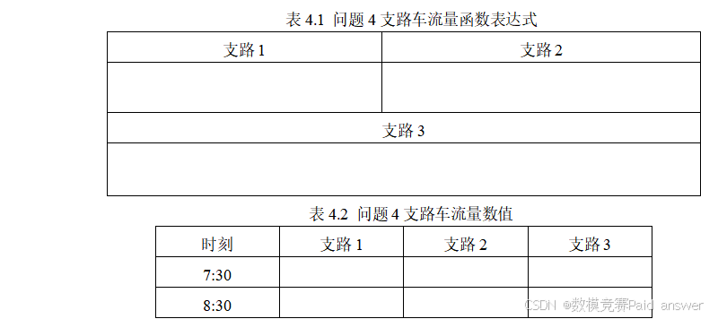
请建立数学模型,根据附件表 4 的数据推测支路 1、支路 2、支路 3 上实际的车流量,使用合适的函数关系来描述各支路上的车流量随时间的变化,并分析结果的误差。在表 4.1 中填入具体的函数表达式,在表 4.2 中分别填入 7:30 和 8:30 这两个时刻各支路上的车流量数值。
问题 5. 在某些时间段内,各支路的车流量具有特定函数变化趋势。因此无需在每个时刻都进行监测,只需在一些关键时刻记录车流量数据,就能够推断出整个时间段内各支路的车流量函数表达式。
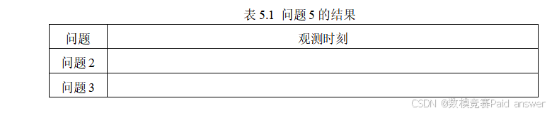
基于问题 2 和问题 3,请建立数学模型并分别回答:为了得到各支路的函数表达式,主路上的监测设备至少需要在 6:58,8:58 时间段内的哪些时刻记录车流量数据?并填入表 5.1。
整体求解过程概述(摘要)
针对问题一,为了从Y型道路主路总流量中推测两条支路流量,首先对表1进行完整性检查、描述性统计与一阶差分诊断。数据在t=30处发生唯一斜率突变,主路在前半段以1.5的离散斜率严格增长,后半段以−0.5的斜率严格下降。鉴于单一总量方程对两条支路的绝对截距与增长斜率存在结构性不可辨识,本文引入最小参数能量规范化准则,在满足支路1严格线性增长、支路2先增后减、连续性与非负性的条件下构建约束分解模型,得到支路1为f₁(t)=3.5+t/3,支路2为分段函数f₂(t)=3.5+7t/6(t≤30)与f₂(t)=38.5−5(t−30)/6(t>30)。重构主路流量的RMSE为0,说明模型与数据完全一致。
针对问题二,考虑到支路1、2存在2分钟传播时滞,支路4具有周期性,本文先进行时标对齐,再通过分段斜率、残差周期回归和候选周期扫描识别出支路3在t=17后稳定、支路4周期为28个采样步长(56分钟)。为了避免重复处理,问题二直接复用统一的数据质量检查结果,并在问题一"总量分解不可辨识"的认识基础上引入非负周期基线与等截距最小范数规范化。最终四支路函数可精确重构表2,RMSE约为4.77×10⁻¹⁵;7:30时四支路流量分别为10.033、18.433、25.033、0,8:30时分别为10.033、27.233、27.033、0。
针对问题三,为了处理信号灯导致的间歇放行与支路1复杂阶段变化,首先依据2分钟传播时滞构造支路1、2的滞后叠加方程,并利用红灯样本与每个绿灯开始时刻的零放行信息识别"基线流量"。由此推得支路2为已知断点的分段线性函数,支路1在s∈(7,23]内为三次多项式,其后经历稳定与线性衰减;支路3则按18分钟周期在各绿灯段内采用线性或常值函数。模型完整复现表3,且支路1峰值出现在s≈18.318。7:30时三支路流量为49.735、18.800、24.250,8:30时为0、44、0。
针对问题四,鉴于观测数据含随机误差且绿灯相位未知,本文将相位识别与参数估计分层处理:首先在9个候选相位上计算非绿灯样本的趋势拟合误差,识别有效放行样本块从t≡2(mod 9)开始,即首个绿灯起始相位为t≡1(mod 9);随后采用断点局部枚举、非负约束和Huber损失构建鲁棒分段回归。估计支路1断点为(9,29,39,49),平台高度22.5635;支路2初始流量19.8544、增长斜率0.8450、后段下降斜率1.2432。模型RMSE为1.9966、R²为0.9904,残差Shapiro-Wilk检验p=0.234,说明误差近似对称且无显著非正态性。7:30时估计三支路流量为5.641、32.529、18.869,8:30时为11.282、23.875、0。
针对问题五,本文从结构可辨识性和实验设计角度统一讨论最少观测。严格而言,若不引入截距规范化、断点、周期和相位等先验,单一主路监测方程始终存在秩亏,任何有限观测集合均无法唯一分离全部支路绝对基线。在本文规范化模型下,问题二设计矩阵秩为6,QR列主元法选得6个代表性观测时刻:7:00、7:12、7:34、7:50、8:30、8:58;问题三设计矩阵秩为18,对应18个最少观测时刻。整体而言,本文形成"数据理解与探索---结构辨识---约束建模---鲁棒估计---误差验证---最优采样"的完整流程,既保证函数趋势与交通机理一致,也明确揭示了单监测点反问题的不可辨识边界。
模型假设:
主路监测值等于相应时刻到达监测点的各支路标准车当量之和;除问题四外不含测量误差。
每2分钟观测值代表该采样时刻附近的等效流量;传播时间2分钟精确对应一个离散步长。
题目给出的"线性增长、线性减少、稳定、周期性、红灯为0"等历史趋势先验真实有效。
各支路流量非负;除信号切换边界外,函数采用连续分段函数。对离散周期模板使用一阶保持插值实现连续延拓。
问题四误差相互独立、中心近似为0,但允许少量较大扰动,因此采用Huber损失而不是完全依赖正态最小二乘。
为了在结构不可辨识时给出可复现的代表性解,采用最小参数能量、非负最小基线或等截距最小范数规范化;该规范化不声称恢复唯一物理真值。
问题五中的最少观测基于前述已经识别的断点、周期和相位;若这些结构先验未知,所需观测数将增加,甚至无法唯一识别。
问题分析:
本题本质上是欠定的函数分解反问题。在每一时刻只观测到一个主路总量,却需要推断多条支路函数。即使趋势类别已知,若多个支路都含常数项或相同基函数,则设计矩阵会出现线性相关,绝对基线不能仅凭总量唯一确定。因此,模型不仅要拟合数据,还必须讨论可辨识性、规范化选择与不确定性。
问题一的斜率突变能够唯一确定主路的两段斜率,却不能唯一确定两支路各自斜率;问题二中稳定支路的常数与其他支路截距互相混淆;问题三借助红灯时支路3为0、支路1早期为0等"结构零值"提高了可辨识性;问题四的噪声与相位未知使普通最小二乘容易被异常扰动和错误相位共同影响。
总体技术路线
为了保证每一步均有明确目的与数学依据,本文采用"数据理解与探索 ➔ 数据预处理 ➔ 特征工程 ➔ 模型构建 ➔ 模型训练与评估 ➔ 结果解释与洞察"的流程,并根据各问关联性避免重复操作。问题二至问题四共享相同的基础数据质量检查和时标定义;后续问题仅在新增的传播、周期、门控或噪声机制上深化。
数据理解与探索:检查工作表结构、缺失值、时间间隔、取值范围,计算均值、标准差、变异系数、偏度、峰度与Shapiro-Wilk检验。
数据预处理:统一t时标,对有2分钟行驶时间的支路进行s=t−1的滞后对齐;问题四保留原始值,不进行会破坏周期突变的移动平均。
特征工程:构造一阶差分、截断线性基函数、铰链函数、周期相位变量、信号灯门控变量及分段函数基。
模型构建:问题一采用变点分段回归与最小能量规范化;问题二采用滞后叠加和周期计算;问题三采用结构零值分离基线与信号流;问题四采用相位枚举与Huber鲁棒约束回归。
模型评估:使用SSE、RMSE、MAE、MAPE、R²、残差偏度峰度、正态性检验和参数敏感性进行验证。
最优采样:将已建立的模型写成设计矩阵,通过矩阵秩判定参数维数,并利用QR主元法选择信息量充足的最少观测行。
模型的建立与求解整体论文缩略图
全部论文请见下方" 只会建模 QQ名片" 点击QQ名片即可
程序代码:
python
from __future__ import annotations
import argparse
import json
import math
import os
import re
import statistics
import zipfile
from dataclasses import dataclass
from pathlib import Path
from typing import Dict, List, Sequence, Tuple
from xml.etree import ElementTree as ET
import matplotlib.pyplot as plt
import numpy as np
from scipy import linalg, stats
from scipy.optimize import least_squares
# ---------- 全局绘图设置 ----------
plt.rcParams["font.sans-serif"] = ["Noto Sans CJK JP", "Noto Sans CJK SC", "SimHei", "DejaVu Sans"]
plt.rcParams["axes.unicode_minus"] = False
plt.rcParams["figure.dpi"] = 140
plt.rcParams["savefig.dpi"] = 180
NS_MAIN = "http://schemas.openxmlformats.org/spreadsheetml/2006/main"
NS_REL = "http://schemas.openxmlformats.org/officeDocument/2006/relationships"
NS_PKG_REL = "http://schemas.openxmlformats.org/package/2006/relationships"
# =========================
# 一、XLSX 轻量读取器
# =========================
def _column_index(cell_ref: str) -> int:
letters = re.match(r"([A-Z]+)", cell_ref).group(1)
idx = 0
for ch in letters:
idx = idx * 26 + ord(ch) - ord("A") + 1
return idx - 1
def read_xlsx(path: str | Path) -> Dict[str, List[List[object]]]:
"""读取 xlsx 中所有工作表,返回 {sheet_name: rows}。"""
path = Path(path)
if not path.exists():
raise FileNotFoundError(f"找不到输入文件:{path}")
with zipfile.ZipFile(path, "r") as zf:
names = set(zf.namelist())
shared: List[str] = []
if "xl/sharedStrings.xml" in names:
root = ET.fromstring(zf.read("xl/sharedStrings.xml"))
for si in root.findall(f"{{{NS_MAIN}}}si"):
texts = [node.text or "" for node in si.iter(f"{{{NS_MAIN}}}t")]
shared.append("".join(texts))
wb_root = ET.fromstring(zf.read("xl/workbook.xml"))
rel_root = ET.fromstring(zf.read("xl/_rels/workbook.xml.rels"))
rel_map = {
rel.attrib["Id"]: rel.attrib["Target"]
for rel in rel_root.findall(f"{{{NS_PKG_REL}}}Relationship")
}
output: Dict[str, List[List[object]]] = {}
sheets_node = wb_root.find(f"{{{NS_MAIN}}}sheets")
for sheet in sheets_node:
sheet_name = sheet.attrib["name"]
rid = sheet.attrib[f"{{{NS_REL}}}id"]
target = rel_map[rid]
sheet_path = "xl/" + target.lstrip("/")
root = ET.fromstring(zf.read(sheet_path))
rows: List[List[object]] = []
for row in root.iter(f"{{{NS_MAIN}}}row"):
values: Dict[int, object] = {}
max_col = -1
for cell in row.findall(f"{{{NS_MAIN}}}c"):
ref = cell.attrib.get("r", "A1")
col = _column_index(ref)
max_col = max(max_col, col)
ctype = cell.attrib.get("t")
value_node = cell.find(f"{{{NS_MAIN}}}v")
inline = cell.find(f"{{{NS_MAIN}}}is")
if inline is not None:
text = "".join(n.text or "" for n in inline.iter(f"{{{NS_MAIN}}}t"))
val: object = text
elif value_node is None:
val = None
else:
raw = value_node.text or ""
if ctype == "s":
val = shared[int(raw)]
elif ctype == "b":
val = raw == "1"
elif ctype in ("str", "inlineStr"):
val = raw
else:
try:
num = float(raw)
val = int(num) if num.is_integer() else num
except ValueError:
val = raw
values[col] = val
rows.append([values.get(i) for i in range(max_col + 1)])
output[sheet_name] = rows
return output
def extract_series(workbook: Dict[str, List[List[object]]]) -> Dict[str, Dict[str, np.ndarray]]:
result = {}
for name, rows in workbook.items():
body = [r for r in rows[1:] if len(r) >= 3 and r[1] is not None and r[2] is not None]
result[name] = {
"moment": np.array([str(r[0]).strip() for r in body], dtype=object),
"t": np.array([float(r[1]) for r in body], dtype=float),
"y": np.array([float(r[2]) for r in body], dtype=float),
}
return result
# =========================
# 二、统计与工具函数
# =========================
def descriptive_statistics(x: np.ndarray) -> Dict[str, float]:
x = np.asarray(x, dtype=float)
q1, median, q3 = np.percentile(x, [25, 50, 75])
shapiro_p = stats.shapiro(x).pvalue if len(x) <= 5000 else float("nan")
return {
"样本量": int(len(x)),
"均值": float(np.mean(x)),
"标准差": float(np.std(x, ddof=1)),
"最小值": float(np.min(x)),
"第一四分位数": float(q1),
"中位数": float(median),
"第三四分位数": float(q3),
"最大值": float(np.max(x)),
"变异系数": float(np.std(x, ddof=1) / np.mean(x)),
"偏度": float(stats.skew(x, bias=False)),
"峰度": float(stats.kurtosis(x, fisher=True, bias=False)),
"Shapiro-Wilk_p值": float(shapiro_p),
}
def metrics(y: np.ndarray, yhat: np.ndarray) -> Dict[str, float]:
y = np.asarray(y, float)
yhat = np.asarray(yhat, float)
e = y - yhat
sse = np.sum(e**2)
sst = np.sum((y - np.mean(y)) ** 2)
return {
"SSE": float(sse),
"MSE": float(np.mean(e**2)),
"RMSE": float(np.sqrt(np.mean(e**2))),
"MAE": float(np.mean(np.abs(e))),
"MAPE(%)": float(np.mean(np.abs(e) / np.maximum(np.abs(y), 1e-8)) * 100),
"R2": float(1 - sse / sst) if sst > 0 else 1.0,
"残差均值": float(np.mean(e)),
"残差标准差": float(np.std(e, ddof=1)),
"残差偏度": float(stats.skew(e, bias=False)),
"残差峰度": float(stats.kurtosis(e, fisher=True, bias=False)),
"残差Shapiro_p值": float(stats.shapiro(e).pvalue),
}
def savefig(path: Path) -> None:
plt.tight_layout()
plt.savefig(path, bbox_inches="tight")
plt.close()
def time_label(t: int) -> str:
minutes = 7 * 60 + 2 * t
return f"{minutes // 60:02d}:{minutes % 60:02d}"
def first_order_hold(t_cont: np.ndarray, samples: np.ndarray, period: int | None = None) -> np.ndarray:
"""一阶保持插值;period 非空时作周期延拓。"""
t_cont = np.asarray(t_cont, float)
if period is None:
grid = np.arange(len(samples))
return np.interp(t_cont, grid, samples)
x = np.mod(t_cont, period)
extended_x = np.arange(period + 1)
extended_y = np.r_[samples[:period], samples[0]]
return np.interp(x, extended_x, extended_y)
# =========================
# 三、问题1
# =========================
def solve_problem1(t: np.ndarray, y: np.ndarray) -> Dict[str, object]:
# 变点通过穷举分段线性回归识别
candidates = []
for tau in range(2, len(t) - 2):
X = np.column_stack([np.ones(len(t)), t, np.maximum(t - tau, 0)])
beta = np.linalg.lstsq(X, y, rcond=None)[0]
yhat = X @ beta
candidates.append((np.sum((y - yhat) ** 2), tau, beta, yhat))
sse, tau, beta, yhat = min(candidates, key=lambda z: z[0])
# 结构不可辨识:以斜率能量与截距能量最小作为规范化选择
# min a^2+(1.5-a)^2+(-0.5-a)^2 -> a=1/3
a1 = 1.0 / 3.0
b1 = 3.5
f1 = b1 + a1 * t
f2 = np.where(t <= tau, 3.5 + 7.0 / 6.0 * t, 38.5 - 5.0 / 6.0 * (t - tau))
fitted = f1 + f2
return {
"change_point": int(tau),
"change_time": time_label(int(tau)),
"main_beta": beta.tolist(),
"branch1": f1,
"branch2": f2,
"fitted": fitted,
"metrics": metrics(y, fitted),
"candidate_sse": np.array([c[0] for c in candidates]),
}
# =========================
# 四、问题2
# =========================
def problem2_f4_samples() -> np.ndarray:
q = np.zeros(28)
q[0:6] = 3.0
q[6:14] = 14.0
q[14:18] = 0.0
q[18:26] = 14.0
q[26:28] = 3.0
return q
def solve_problem2(t: np.ndarray, y: np.ndarray) -> Dict[str, object]:
s = t - 1
c = 30.1 / 3.0
f1 = np.full_like(t, c)
f2 = np.where(s <= 24, c + 0.6 * s,
np.where(s <= 37, c + 14.4, c + 14.4 + 0.4 * (s - 37)))
f3 = np.where(t <= 17, c + t, c + 17)
q = problem2_f4_samples()
f4 = q[(t.astype(int) % 28)]
fitted = f1 + f2 + f3 + f4
# 周期识别:去趋势后计算候选周期的均方误差
g1 = np.minimum(s, 24)
g2 = np.maximum(s - 37, 0)
h = np.minimum(t, 17)
period_scores = []
for p in range(2, 31):
phase_cols = [(t.astype(int) % p == j).astype(float) for j in range(1, p)]
X = np.column_stack([np.ones(len(t)), g1, g2, h] + phase_cols)
b = np.linalg.lstsq(X, y, rcond=None)[0]
period_scores.append(np.sqrt(np.mean((y - X @ b) ** 2)))
return {
"branch1": f1, "branch2": f2, "branch3": f3, "branch4": f4,
"fitted": fitted, "metrics": metrics(y, fitted),
"period_scores": np.array(period_scores), "periods": np.arange(2, 31),
"q": q,
}
# =========================
# 五、问题3
# =========================
def p3_branch1(s: np.ndarray) -> np.ndarray:
s = np.asarray(s, float)
cubic = -0.01 * s**3 - 0.03 * s**2 + 11.165 * s - 73.255
return np.where(s <= 7, 0,
np.where(s <= 23, cubic,
np.where(s <= 32, 46,
np.where(s <= 42, 46 - 4.6 * (s - 32), 0))))
def p3_branch2(s: np.ndarray) -> np.ndarray:
s = np.asarray(s, float)
return np.where(s <= 35, 1.2 * s + 2,
np.where(s <= 47, 44, 44 - 0.85 * (s - 47)))
def p3_branch3_discrete(t: np.ndarray) -> np.ndarray:
t = np.asarray(t, int)
out = np.zeros_like(t, dtype=float)
blocks = [
(4, 8, 29.0, 1.5),
(13, 17, 25.55, -0.65),
(22, 26, 27.4, -0.8),
(31, 35, 24.8, 0.8),
(40, 44, 19.0, 0.0),
(49, 53, 39.0, 1.0),
(58, 62, 17.0, 0.0),
]
for left, right, intercept, slope in blocks:
m = (t >= left) & (t <= right)
out[m] = intercept + slope * (t[m] - left)
return out
def solve_problem3(t: np.ndarray, y: np.ndarray) -> Dict[str, object]:
s = t - 1
f1 = p3_branch1(s)
f2 = p3_branch2(s)
f3 = p3_branch3_discrete(t)
fitted = f1 + f2 + f3
peak_t = (-12 + math.sqrt(12**2 + 4 * 6 * 2233)) / 12
return {
"branch1": f1, "branch2": f2, "branch3": f3,
"fitted": fitted, "metrics": metrics(y, fitted),
"branch1_peak_s": peak_t,
"branch1_peak_value": float(p3_branch1(np.array([peak_t]))[0]),
}
# =========================
# 六、问题4:相位搜索 + 鲁棒约束回归
# =========================
def p4_b1_shape(s: np.ndarray, a: int, b: int, c: int, d: int) -> np.ndarray:
s = np.asarray(s, float)
z = np.zeros_like(s)
m = (s > a) & (s <= b)
z[m] = (s[m] - a) / (b - a)
m = (s > b) & (s <= c)
z[m] = 1
m = (s > c) & (s < d)
z[m] = (d - s[m]) / (d - c)
return z
def p4_design(t: np.ndarray, phase_positive_start: int,
breakpoints: Tuple[int, int, int, int]) -> Tuple[np.ndarray, List[int]]:
t = np.asarray(t, int)
s = t - 1
inc = np.minimum(np.maximum(s + 1, 0), 18)
dec = np.maximum(s - 35, 0)
cols = [np.ones(len(t)), inc, -dec, p4_b1_shape(s, *breakpoints)]
starts: List[int] = []
for k in range(-2, 20):
st = phase_positive_start + 9 * k
idx = np.where((t >= st) & (t <= st + 4))[0]
if len(idx) == 0:
continue
starts.append(st)
left = np.zeros(len(t))
right = np.zeros(len(t))
x = (t[idx] - st) / 4.0
left[idx] = 1 - x
right[idx] = x
cols.extend([left, right])
return np.column_stack(cols), starts
def fit_p4_model(t: np.ndarray, y: np.ndarray,
phase_positive_start: int,
breakpoints: Tuple[int, int, int, int],
f_scale: float = 2.0) -> Dict[str, object]:
X, starts = p4_design(t, phase_positive_start, breakpoints)
x0 = np.linalg.lstsq(X, y, rcond=None)[0]
x0[:4] = np.maximum(x0[:4], 1e-3)
x0[4:] = np.maximum(x0[4:], 0.1)
lb = np.full(X.shape[1], -np.inf)
ub = np.full(X.shape[1], np.inf)
lb[:] = 0.0
fit = least_squares(lambda b: X @ b - y, x0, bounds=(lb, ub),
loss="huber", f_scale=f_scale, max_nfev=3000)
yhat = X @ fit.x
residual = y - yhat
huber_score = float(np.mean(2 * (np.sqrt(1 + (residual / f_scale) ** 2) - 1)))
return {
"coef": fit.x, "fitted": yhat, "residual": residual,
"starts": starts, "X": X, "huber_score": huber_score,
"metrics": metrics(y, yhat),
}
def solve_problem4(t: np.ndarray, y: np.ndarray) -> Dict[str, object]:
# 1) 相位识别:以非绿灯样本上的受限趋势模型 RMSE 为判据
phase_scores = []
for r0 in range(9):
green = ((t.astype(int) - r0) % 9 <= 4)
red = ~green
# 使用较宽松的核心趋势候选,固定一组近似断点即可突出相位差异
X = np.column_stack([
np.ones(np.sum(red)),
np.minimum(np.maximum((t[red] - 1) + 1, 0), 18),
-np.maximum((t[red] - 1) - 35, 0),
p4_b1_shape(t[red] - 1, 9, 29, 39, 49),
])
b = np.linalg.lstsq(X, y[red], rcond=None)[0]
phase_scores.append(float(np.sqrt(np.mean((y[red] - X @ b) ** 2))))
best_phase = int(np.argmin(phase_scores)) # 非零流量块起始相位
# 2) 局部枚举断点并使用 Huber 损失选择
candidate_rows = []
for a in range(8, 11):
for b in range(27, 31):
for c in range(38, 41):
for d in range(47, 51):
if not (a < b <= c < d):
continue
fit = fit_p4_model(t, y, best_phase, (a, b, c, d))
candidate_rows.append((fit["huber_score"], a, b, c, d, fit))
best = min(candidate_rows, key=lambda z: z[0])
_, a, b, c, d, fit = best
coef = fit["coef"]
s = t - 1
u, v, w, H = coef[:4]
f1 = H * p4_b1_shape(s, a, b, c, d)
f2 = u + v * np.minimum(np.maximum(s + 1, 0), 18) - w * np.maximum(s - 35, 0)
f3 = fit["fitted"] - f1 - f2
# Huber 权重(用于稳健性可视化)
r = fit["residual"]
delta = 2.0
weights = np.where(np.abs(r) <= delta, 1.0, delta / np.abs(r))
return {
"phase_scores": np.array(phase_scores),
"phase_positive_start": best_phase,
"green_onset_phase": (best_phase - 1) % 9,
"breakpoints": [a, b, c, d],
"coef": coef,
"starts": fit["starts"],
"branch1": f1, "branch2": f2, "branch3": f3,
"fitted": fit["fitted"], "residual": r,
"weights": weights, "metrics": fit["metrics"],
"candidate_scores": sorted([(float(z[0]), z[1], z[2], z[3], z[4]) for z in candidate_rows])[:30],
}
# =========================
# 七、问题5:可辨识性与最少观测设计
# =========================
def solve_problem5() -> Dict[str, object]:
# 问题2:规范化模型的6维可辨识参数
t = np.arange(60)
s = t - 1
phase = t % 28
cat1 = (((phase >= 6) & (phase <= 13)) | ((phase >= 18) & (phase <= 25))).astype(float)
cat2 = ((phase >= 14) & (phase <= 17)).astype(float)
X2 = np.column_stack([
np.ones(60), np.minimum(s, 24), np.maximum(s - 37, 0),
np.minimum(t, 17), cat1, cat2,
])
_, _, piv2 = linalg.qr(X2.T, pivoting=True, mode="economic")
selected2 = sorted(map(int, piv2[:np.linalg.matrix_rank(X2)]))
# 问题3:3个支路1基函数 + 3个支路2基函数 + 12个绿灯段参数 = 18维
def b1_component(power: int) -> np.ndarray:
x = s.astype(float)
raw = (x - 7) * x**power
v23 = (23 - 7) * 23**power
out = np.zeros(60)
m = (x > 7) & (x <= 23)
out[m] = raw[m]
m = (x > 23) & (x <= 32)
out[m] = v23
m = (x > 32) & (x <= 42)
out[m] = v23 * (42 - x[m]) / 10
return out
columns = [
b1_component(2), b1_component(1), b1_component(0),
np.ones(60), np.minimum(s, 35), -np.maximum(s - 47, 0),
]
starts = [4, 13, 22, 31, 40, 49, 58]
stable = {40, 58}
for st in starts:
idx = np.arange(st, min(st + 5, 60))
c0 = np.zeros(60); c0[idx] = 1
columns.append(c0)
if st not in stable:
c1 = np.zeros(60); c1[idx] = idx - st
columns.append(c1)
X3 = np.column_stack(columns)
_, _, piv3 = linalg.qr(X3.T, pivoting=True, mode="economic")
selected3 = sorted(map(int, piv3[:np.linalg.matrix_rank(X3)]))
return {
"rank_problem2": int(np.linalg.matrix_rank(X2)),
"selected_problem2": selected2,
"times_problem2": [time_label(i) for i in selected2],
"singular_problem2": np.linalg.svd(X2, compute_uv=False).tolist(),
"X2": X2,
"rank_problem3": int(np.linalg.matrix_rank(X3)),
"selected_problem3": selected3,
"times_problem3": [time_label(i) for i in selected3],
"singular_problem3": np.linalg.svd(X3, compute_uv=False).tolist(),
"X3": X3,
"strict_identifiability_note": (
"若不引入截距规范化、已知断点/周期/信号相位等先验,则单一主路监测方程存在结构性秩亏,"
"任何有限观测集合均不能唯一分离所有支路的绝对基线。"
),
}
# =========================
# 八、绘图
# =========================
def create_figures(series: Dict[str, Dict[str, np.ndarray]], results: Dict[str, object], out: Path) -> None:
out.mkdir(parents=True, exist_ok=True)
names = list(series.keys())
# 图1:四组原始数据
plt.figure(figsize=(10, 5.5))
for name in names:
d = series[name]
plt.plot(d["t"], d["y"], marker="o", markersize=2.5, linewidth=1.2, label=name.split()[0])
plt.xlabel("时间变量 t(每单位为2分钟,7:00对应t=0)")
plt.ylabel("主路车流量")
plt.title("附件四组主路车流量的整体时序特征")
plt.legend(ncol=4)
plt.grid(alpha=0.25)
savefig(out / "fig01_四组原始数据.png")
# 图2:描述性统计箱线图
plt.figure(figsize=(8.5, 5.2))
plt.boxplot([series[n]["y"] for n in names], tick_labels=[n.split()[0] for n in names], showmeans=True)
plt.ylabel("主路车流量")
plt.title("四组观测数据的箱线图与均值位置")
plt.grid(axis="y", alpha=0.25)
savefig(out / "fig02_箱线图.png")
# 图3:差分序列
plt.figure(figsize=(10, 5.8))
for name in names:
d = series[name]
plt.plot(d["t"][1:], np.diff(d["y"]), linewidth=1.1, label=name.split()[0])
plt.axhline(0, linewidth=0.8)
plt.xlabel("时间变量 t")
plt.ylabel("一阶差分 Δy")
plt.title("一阶差分用于识别斜率、突变与周期结构")
plt.legend(ncol=4)
plt.grid(alpha=0.25)
savefig(out / "fig03_一阶差分.png")
# 图4:偏度峰度散点
skews = [stats.skew(series[n]["y"], bias=False) for n in names]
kurts = [stats.kurtosis(series[n]["y"], fisher=True, bias=False) for n in names]
plt.figure(figsize=(7.5, 5.2))
plt.scatter(skews, kurts, s=70)
for i, n in enumerate(names):
plt.annotate(n.split()[0], (skews[i], kurts[i]), xytext=(5, 5), textcoords="offset points")
plt.axvline(0, linewidth=0.8); plt.axhline(0, linewidth=0.8)
plt.xlabel("偏度")
plt.ylabel("超额峰度")
plt.title("主路流量分布的偏度---峰度诊断")
plt.grid(alpha=0.25)
savefig(out / "fig04_偏度峰度.png")
# 问题1
r1 = results["problem1"]; d1 = series[names[0]]
plt.figure(figsize=(10, 5.2))
plt.plot(d1["t"], d1["y"], "o", markersize=3, label="观测主路3")
plt.plot(d1["t"], r1["fitted"], linewidth=2, label="分段线性重构")
plt.axvline(r1["change_point"], linestyle="--", label=f"变点 t={r1['change_point']}")
plt.xlabel("t"); plt.ylabel("车流量"); plt.title("问题1:变点识别与主路拟合")
plt.legend(); plt.grid(alpha=0.25)
savefig(out / "fig05_问题1变点拟合.png")
plt.figure(figsize=(10, 5.2))
plt.plot(d1["t"], r1["branch1"], label="支路1")
plt.plot(d1["t"], r1["branch2"], label="支路2")
plt.plot(d1["t"], r1["branch1"] + r1["branch2"], linestyle="--", label="支路和")
plt.xlabel("t"); plt.ylabel("车流量"); plt.title("问题1:最小能量规范化后的支路分解")
plt.legend(); plt.grid(alpha=0.25)
savefig(out / "fig06_问题1支路分解.png")
plt.figure(figsize=(9, 4.8))
tau = np.arange(2, 58)
plt.semilogy(tau, np.maximum(r1["candidate_sse"], 1e-14))
plt.axvline(r1["change_point"], linestyle="--")
plt.xlabel("候选变点 τ"); plt.ylabel("SSE(对数尺度)")
plt.title("问题1:分段回归变点目标函数")
plt.grid(alpha=0.25)
savefig(out / "fig07_问题1变点目标.png")
# 问题2
r2 = results["problem2"]; d2 = series[names[1]]
plt.figure(figsize=(9, 4.8))
plt.plot(r2["periods"], r2["period_scores"], marker="o", markersize=3)
plt.axvline(28, linestyle="--", label="最优周期28")
plt.xlabel("候选周期(t单位)"); plt.ylabel("周期回归RMSE")
plt.title("问题2:支路4周期长度识别")
plt.legend(); plt.grid(alpha=0.25)
savefig(out / "fig08_问题2周期识别.png")
plt.figure(figsize=(10, 5.7))
plt.plot(d2["t"], d2["y"], "o", markersize=3, label="观测主路5")
plt.plot(d2["t"], r2["fitted"], linewidth=1.8, label="支路和")
plt.xlabel("t"); plt.ylabel("车流量"); plt.title("问题2:主路重构验证")
plt.legend(); plt.grid(alpha=0.25)
savefig(out / "fig09_问题2主路重构.png")
plt.figure(figsize=(10, 6))
for key, lab in [("branch1", "支路1"), ("branch2", "支路2"), ("branch3", "支路3"), ("branch4", "支路4")]:
plt.plot(d2["t"], r2[key], label=lab)
plt.xlabel("t"); plt.ylabel("车流量"); plt.title("问题2:四条支路的函数性变化")
plt.legend(ncol=2); plt.grid(alpha=0.25)
savefig(out / "fig10_问题2支路分解.png")
plt.figure(figsize=(9, 4.8))
plt.step(np.arange(28), r2["q"], where="mid")
plt.xlabel("周期相位 r=t mod 28"); plt.ylabel("支路4流量")
plt.title("问题2:支路4的28步周期样本模板")
plt.grid(alpha=0.25)
savefig(out / "fig11_问题2周期模板.png")
# 问题3
r3 = results["problem3"]; d3 = series[names[2]]
plt.figure(figsize=(10, 5.5))
plt.plot(d3["t"], d3["y"], "o", markersize=3, label="观测主路4")
plt.plot(d3["t"], r3["fitted"], linewidth=1.8, label="模型重构")
plt.xlabel("t"); plt.ylabel("车流量"); plt.title("问题3:含信号灯控制的主路重构")
plt.legend(); plt.grid(alpha=0.25)
savefig(out / "fig12_问题3主路重构.png")
plt.figure(figsize=(10, 6))
for key, lab in [("branch1", "支路1"), ("branch2", "支路2"), ("branch3", "支路3(信号控制)")]:
plt.plot(d3["t"], r3[key], label=lab)
plt.xlabel("t"); plt.ylabel("车流量"); plt.title("问题3:三条支路车流量分解")
plt.legend(); plt.grid(alpha=0.25)
savefig(out / "fig13_问题3支路分解.png")
s_dense = np.linspace(-1, 45, 600)
f_dense = p3_branch1(s_dense)
plt.figure(figsize=(9.5, 5.2))
plt.plot(s_dense, f_dense, linewidth=2)
plt.axvline(r3["branch1_peak_s"], linestyle="--", label=f"峰值位置 s={r3['branch1_peak_s']:.3f}")
plt.xlabel("支路时标 s"); plt.ylabel("支路1流量")
plt.title("问题3:支路1的增长---减少---稳定---衰减结构")
plt.legend(); plt.grid(alpha=0.25)
savefig(out / "fig14_问题3支路1形态.png")
plt.figure(figsize=(10, 4.8))
green = (r3["branch3"] > 0).astype(float)
plt.step(d3["t"], green, where="mid", label="有效放行状态")
plt.plot(d3["t"], r3["branch3"] / max(np.max(r3["branch3"]), 1), label="归一化支路3流量")
plt.xlabel("t"); plt.ylabel("状态/归一化流量")
plt.title("问题3:信号周期与支路3放行流量")
plt.legend(); plt.grid(alpha=0.25)
savefig(out / "fig15_问题3信号状态.png")
# 问题4
r4 = results["problem4"]; d4 = series[names[3]]
plt.figure(figsize=(8.5, 4.8))
plt.plot(np.arange(9), r4["phase_scores"], marker="o")
plt.axvline(r4["phase_positive_start"], linestyle="--", label=f"最优非零块相位={r4['phase_positive_start']}")
plt.xlabel("候选相位"); plt.ylabel("非绿灯样本RMSE")
plt.title("问题4:未知信号灯相位的离散搜索")
plt.legend(); plt.grid(alpha=0.25)
savefig(out / "fig16_问题4相位识别.png")
plt.figure(figsize=(10, 5.5))
plt.plot(d4["t"], d4["y"], "o", markersize=3, label="含误差观测")
plt.plot(d4["t"], r4["fitted"], linewidth=1.8, label="Huber鲁棒重构")
plt.xlabel("t"); plt.ylabel("车流量"); plt.title("问题4:含误差数据的鲁棒拟合")
plt.legend(); plt.grid(alpha=0.25)
savefig(out / "fig17_问题4鲁棒拟合.png")
plt.figure(figsize=(10, 6))
for key, lab in [("branch1", "支路1"), ("branch2", "支路2"), ("branch3", "支路3")]:
plt.plot(d4["t"], r4[key], label=lab)
plt.xlabel("t"); plt.ylabel("车流量"); plt.title("问题4:鲁棒估计得到的支路实际流量")
plt.legend(); plt.grid(alpha=0.25)
savefig(out / "fig18_问题4支路分解.png")
plt.figure(figsize=(10, 4.8))
plt.stem(d4["t"], r4["residual"], basefmt=" ")
plt.axhline(0, linewidth=0.8)
plt.xlabel("t"); plt.ylabel("残差")
plt.title("问题4:鲁棒模型残差时序")
plt.grid(alpha=0.25)
savefig(out / "fig19_问题4残差时序.png")
plt.figure(figsize=(8.5, 4.8))
plt.hist(r4["residual"], bins=12, density=True, alpha=0.7)
xx = np.linspace(np.min(r4["residual"]), np.max(r4["residual"]), 200)
mu, sd = np.mean(r4["residual"]), np.std(r4["residual"], ddof=1)
plt.plot(xx, stats.norm.pdf(xx, mu, sd), linewidth=1.8, label="同均值方差正态密度")
plt.xlabel("残差"); plt.ylabel("密度"); plt.title("问题4:残差分布诊断")
plt.legend(); plt.grid(alpha=0.25)
savefig(out / "fig20_问题4残差直方图.png")
plt.figure(figsize=(6.5, 5.5))
stats.probplot(r4["residual"], dist="norm", plot=plt)
plt.title("问题4:残差正态Q-Q图")
savefig(out / "fig21_问题4残差QQ.png")
plt.figure(figsize=(10, 4.8))
plt.plot(d4["t"], r4["weights"], marker="o", markersize=3)
plt.xlabel("t"); plt.ylabel("Huber权重")
plt.title("问题4:异常扰动样本的自适应降权")
plt.ylim(0, 1.05); plt.grid(alpha=0.25)
savefig(out / "fig22_问题4Huber权重.png")
# 问题5
r5 = results["problem5"]
plt.figure(figsize=(10, 4.5))
plt.imshow(r5["X2"].T, aspect="auto", interpolation="nearest")
plt.colorbar(label="设计矩阵元素")
plt.xlabel("候选观测时刻索引"); plt.ylabel("参数基函数")
plt.title("问题5:问题2规范化模型的设计矩阵")
savefig(out / "fig23_问题5问题2设计矩阵.png")
plt.figure(figsize=(10, 4.8))
plt.scatter(np.arange(60), np.zeros(60), s=12, label="候选时刻")
plt.scatter(r5["selected_problem2"], np.zeros(len(r5["selected_problem2"])), s=80, marker="|", label="问题2最少观测")
plt.scatter(r5["selected_problem3"], np.ones(len(r5["selected_problem3"])), s=80, marker="|", label="问题3最少观测")
plt.yticks([0, 1], ["问题2", "问题3"])
plt.xlabel("t"); plt.title("问题5:QR主元法选择的代表性最少观测时刻")
plt.legend(); plt.grid(axis="x", alpha=0.25)
savefig(out / "fig24_问题5观测时刻.png")
plt.figure(figsize=(8.8, 4.8))
s2 = np.asarray(r5["singular_problem2"])
s3 = np.asarray(r5["singular_problem3"])
plt.semilogy(np.arange(1, len(s2) + 1), s2, marker="o", label="问题2")
plt.semilogy(np.arange(1, len(s3) + 1), s3, marker="o", label="问题3")
plt.xlabel("奇异值序号"); plt.ylabel("奇异值(对数尺度)")
plt.title("问题5:设计矩阵奇异值与可辨识维数")
plt.legend(); plt.grid(alpha=0.25)
savefig(out / "fig25_问题5奇异值.png")
# 扩展诊断图:问题1可行解族与规范化
a_grid = np.linspace(0.001, 1.499, 500)
J = a_grid**2 + (1.5-a_grid)**2 + (-0.5-a_grid)**2
plt.figure(figsize=(8.8, 4.8))
plt.plot(a_grid, J)
plt.axvline(1/3, linestyle="--", label="最小能量斜率 a=1/3")
plt.xlabel("支路1斜率 a"); plt.ylabel("斜率能量 J(a)")
plt.title("问题1:可行斜率族与最小能量规范化")
plt.legend(); plt.grid(alpha=0.25)
savefig(out / "fig26_问题1规范化目标.png")
# 问题2:去趋势后的周期成分
nonperiod = r2["branch1"] + r2["branch2"] + r2["branch3"]
plt.figure(figsize=(10, 4.8))
plt.plot(d2["t"], d2["y"]-nonperiod, marker="o", markersize=3, label="去趋势残差")
plt.plot(d2["t"], r2["branch4"], linestyle="--", label="识别的周期支路4")
plt.xlabel("t"); plt.ylabel("周期成分")
plt.title("问题2:去除非周期趋势后的周期模板验证")
plt.legend(); plt.grid(alpha=0.25)
savefig(out / "fig27_问题2去趋势周期.png")
# 问题2:未规范化截距设计矩阵的秩亏
X_un = np.column_stack([np.ones(60), np.ones(60), np.ones(60),
np.minimum(d2["t"]-1,24), np.maximum((d2["t"]-1)-37,0),
np.minimum(d2["t"],17),
(((d2["t"].astype(int)%28>=6)&(d2["t"].astype(int)%28<=13)) |
((d2["t"].astype(int)%28>=18)&(d2["t"].astype(int)%28<=25))).astype(float),
((d2["t"].astype(int)%28>=14)&(d2["t"].astype(int)%28<=17)).astype(float)])
su = np.linalg.svd(X_un, compute_uv=False)
plt.figure(figsize=(8.6, 4.8))
plt.semilogy(np.arange(1,len(su)+1), np.maximum(su,1e-15), marker="o")
plt.xlabel("奇异值序号"); plt.ylabel("奇异值(对数尺度)")
plt.title("问题2:分离三个截距时的设计矩阵秩亏")
plt.grid(alpha=0.25)
savefig(out / "fig28_问题2截距秩亏.png")
# 问题3:结构零值用于提取基线
zero_mask = np.isclose(r3["branch3"],0)
plt.figure(figsize=(10,5.0))
plt.plot(d3["t"], r3["branch1"]+r3["branch2"], label="支路1+支路2基线")
plt.scatter(d3["t"][zero_mask], d3["y"][zero_mask], s=30, label="红灯/启动边界观测")
plt.xlabel("t"); plt.ylabel("流量")
plt.title("问题3:利用支路3结构零值识别基线流量")
plt.legend(); plt.grid(alpha=0.25)
savefig(out / "fig29_问题3基线提取.png")
# 问题3:各绿灯块的局部线性形态
plt.figure(figsize=(10,5.2))
for st in [4,13,22,31,40,49,58]:
idx=(d3["t"]>=st)&(d3["t"]<=min(st+4,59))
plt.plot(d3["t"][idx]-st, r3["branch3"][idx], marker="o", label=f"起点t={st}")
plt.xlabel("绿灯块内相对时标"); plt.ylabel("支路3流量")
plt.title("问题3:不同绿灯放行块的线性/稳定形态")
plt.legend(ncol=3,fontsize=8); plt.grid(alpha=0.25)
savefig(out / "fig30_问题3绿灯块比较.png")
# 问题4:断点候选的Huber得分
cand=np.array(r4["candidate_scores"],dtype=float)
plt.figure(figsize=(9.2,5.0))
plt.plot(np.arange(1,len(cand)+1), cand[:,0], marker="o", markersize=3)
plt.xlabel("按得分排序的候选断点组合"); plt.ylabel("平均Huber目标")
plt.title("问题4:前30组断点候选的鲁棒目标函数")
plt.grid(alpha=0.25)
savefig(out / "fig31_问题4断点敏感性.png")
# 问题4:固定结构下的留一法核心参数稳定性(线性最小二乘近似)
Xfull,_=p4_design(d4["t"].astype(int), r4["phase_positive_start"], tuple(r4["breakpoints"]))
loo=[]
for drop in range(60):
mask=np.ones(60,dtype=bool); mask[drop]=False
b=np.linalg.lstsq(Xfull[mask],d4["y"][mask],rcond=None)[0]
loo.append(b[:4])
loo=np.array(loo)
plt.figure(figsize=(10,5.2))
labels=["u","v","w","H"]
for j in range(4):
z=(loo[:,j]-np.mean(loo[:,j]))/max(np.std(loo[:,j],ddof=1),1e-12)
plt.plot(np.arange(60),z,label=labels[j])
plt.xlabel("被删除样本索引"); plt.ylabel("标准化参数偏移")
plt.title("问题4:留一法核心参数稳定性诊断")
plt.legend(); plt.grid(alpha=0.25)
savefig(out / "fig32_问题4留一稳定性.png")
# 问题4:残差自相关
e=r4["residual"]-np.mean(r4["residual"])
acf=[]
for lag in range(16):
acf.append(1.0 if lag==0 else np.corrcoef(e[:-lag],e[lag:])[0,1])
plt.figure(figsize=(8.8,4.8))
plt.stem(np.arange(16),acf,basefmt=" ")
bound=1.96/np.sqrt(len(e))
plt.axhline(bound,linestyle="--"); plt.axhline(-bound,linestyle="--")
plt.xlabel("滞后阶数"); plt.ylabel("样本自相关")
plt.title("问题4:残差自相关函数")
plt.grid(alpha=0.25)
savefig(out / "fig33_问题4残差ACF.png")
# 问题5:完整设计与最少设计的条件数
conds=[np.linalg.cond(r5["X2"]),np.linalg.cond(r5["X2"][r5["selected_problem2"]]),
np.linalg.cond(r5["X3"]),np.linalg.cond(r5["X3"][r5["selected_problem3"]])]
plt.figure(figsize=(9.2,4.8))
plt.bar(["问题2完整","问题2最少","问题3完整","问题3最少"],conds)
plt.yscale("log")
plt.ylabel("2-范数条件数(对数尺度)")
plt.title("问题5:最少采样与完整采样的数值条件比较")
plt.grid(axis="y",alpha=0.25)
savefig(out / "fig34_问题5条件数.png")
# 全题模型性能摘要
rmses=[results[f"problem{i}"]["metrics"]["RMSE"] for i in range(1,5)]
r2s=[results[f"problem{i}"]["metrics"]["R2"] for i in range(1,5)]
plt.figure(figsize=(8.8,4.8))
plt.bar(["问题1","问题2","问题3","问题4"],np.maximum(rmses,1e-15))
plt.yscale("log")
plt.ylabel("RMSE(对数尺度)")
plt.title("问题1---4模型重构误差比较")
plt.grid(axis="y",alpha=0.25)
savefig(out / "fig35_全题RMSE比较.png")
# =========================
# 九、输出表格与主程序
# =========================
def write_csv(path: Path, headers: Sequence[str], rows: Sequence[Sequence[object]]) -> None:
def esc(v: object) -> str:
s = str(v)
if any(ch in s for ch in [",", "\n", '"']):
s = '"' + s.replace('"', '""') + '"'
return s
with path.open("w", encoding="utf-8-sig") as f:
f.write(",".join(map(esc, headers)) + "\n")
for row in rows:
f.write(",".join(map(esc, row)) + "\n")
def json_ready(obj):
if isinstance(obj, np.ndarray):
return obj.tolist()
if isinstance(obj, (np.integer, np.floating)):
return obj.item()
if isinstance(obj, dict):
return {k: json_ready(v) for k, v in obj.items() if k not in {"X", "X2", "X3"}}
if isinstance(obj, (list, tuple)):
return [json_ready(v) for v in obj]
return obj
def main() -> None:
parser = argparse.ArgumentParser(description="支路车流量数学建模完整复现实验")
parser.add_argument("--input", default="附件.xlsx", help="附件xlsx路径")
parser.add_argument("--output", default="建模输出", help="输出目录")
args = parser.parse_args()
output = Path(args.output)
figures = output / "figures"
output.mkdir(parents=True, exist_ok=True)
workbook = read_xlsx(args.input)
series = extract_series(workbook)
names = list(series.keys())
if len(names) < 4:
raise ValueError("附件至少应包含表1---表4四个工作表。")
stats_all = {name: descriptive_statistics(series[name]["y"]) for name in names}
results = {
"problem1": solve_problem1(series[names[0]]["t"], series[names[0]]["y"]),
"problem2": solve_problem2(series[names[1]]["t"], series[names[1]]["y"]),
"problem3": solve_problem3(series[names[2]]["t"], series[names[2]]["y"]),
"problem4": solve_problem4(series[names[3]]["t"], series[names[3]]["y"]),
"problem5": solve_problem5(),
}
create_figures(series, results, figures)
# 描述性统计表
stat_headers = ["工作表"] + list(next(iter(stats_all.values())).keys())
stat_rows = [[name] + [stats_all[name][h] for h in stat_headers[1:]] for name in names]
write_csv(output / "描述性统计.csv", stat_headers, stat_rows)
# 问题1---4分支结果明细
for i in range(1, 5):
r = results[f"problem{i}"]
d = series[names[i - 1]]
branch_keys = [k for k in ["branch1", "branch2", "branch3", "branch4"] if k in r]
rows = []
for j, tv in enumerate(d["t"].astype(int)):
rows.append([time_label(tv), tv, d["y"][j]] + [r[k][j] for k in branch_keys] + [r["fitted"][j], d["y"][j] - r["fitted"][j]])
write_csv(output / f"问题{i}_逐时刻结果.csv",
["时刻", "t", "观测主路"] + branch_keys + ["模型主路", "残差"], rows)
# 关键时刻结果
key_rows = []
for p in [2, 3, 4]:
r = results[f"problem{p}"]
for tv in [15, 45]:
vals = [r[k][tv] for k in ["branch1", "branch2", "branch3", "branch4"] if k in r]
key_rows.append([f"问题{p}", time_label(tv), tv] + vals)
write_csv(output / "关键时刻支路流量.csv", ["问题", "时刻", "t", "支路1", "支路2", "支路3", "支路4(若有)"], key_rows)
summary = {
"descriptive_statistics": stats_all,
"results": results,
}
with (output / "结果汇总.json").open("w", encoding="utf-8") as f:
json.dump(json_ready(summary), f, ensure_ascii=False, indent=2)
print("计算完成。")
print(f"输出目录:{output.resolve()}")
print("问题2最少观测时刻:", results["problem5"]["times_problem2"])
print("问题3最少观测时刻:", results["problem5"]["times_problem3"])
print("问题4RMSE:", results["problem4"]["metrics"]["RMSE"])
if __name__ == "__main__":
main()