如何解决数据预测问题？用线性回归建模实现精准预测

数据预测总是不准？用线性回归建模实现精准预测

关键词：线性回归、最小二乘法、正规方程、梯度下降、回归预测

---

目录

• 一、线性回归：最基础却最实用的预测模型
  • [1.1 什么是线性回归？](#1.1 什么是线性回归？ "#11-%E4%BB%80%E4%B9%88%E6%98%AF%E7%BA%BF%E6%80%A7%E5%9B%9E%E5%BD%92")
  • [1.2 一元 vs 多元线性回归](#1.2 一元 vs 多元线性回归 "#12-%E4%B8%80%E5%85%83-vs-%E5%A4%9A%E5%85%83%E7%BA%BF%E6%80%A7%E5%9B%9E%E5%BD%92")
  • [1.3 线性回归能用在哪些场景？](#1.3 线性回归能用在哪些场景？ "#13-%E7%BA%BF%E6%80%A7%E5%9B%9E%E5%BD%92%E8%83%BD%E7%94%A8%E5%9C%A8%E5%93%AA%E4%BA%9B%E5%9C%BA%E6%99%AF")
• 二、线性回归求解：从损失函数到最优解
  • [2.1 损失函数：MSE与MAE怎么选？](#2.1 损失函数：MSE与MAE怎么选？ "#21-%E6%8D%9F%E5%A4%B1%E5%87%BD%E6%95%B0mse%E4%B8%8Emae%E6%80%8E%E4%B9%88%E9%80%89")
  • [2.2 最小二乘法与解析解](#2.2 最小二乘法与解析解 "#22-%E6%9C%80%E5%B0%8F%E4%BA%8C%E4%B9%98%E6%B3%95%E4%B8%8E%E8%A7%A3%E6%9E%90%E8%A7%A3")
  • [2.3 正规方程法：直接算出最优参数](#2.3 正规方程法：直接算出最优参数 "#23-%E6%AD%A3%E8%A7%84%E6%96%B9%E7%A8%8B%E6%B3%95%E7%9B%B4%E6%8E%A5%E7%AE%97%E5%87%BA%E6%9C%80%E4%BC%98%E5%8F%82%E6%95%B0")
  • [2.4 梯度下降法：迭代逼近最优解](#2.4 梯度下降法：迭代逼近最优解 "#24-%E6%A2%AF%E5%BA%A6%E4%B8%8B%E9%99%8D%E6%B3%95%E8%BF%AD%E4%BB%A3%E9%80%BC%E8%BF%91%E6%9C%80%E4%BC%98%E8%A7%A3")
  • [2.5 学习率怎么选？太大太小都不行](#2.5 学习率怎么选？太大太小都不行 "#25-%E5%AD%A6%E4%B9%A0%E7%8E%87%E6%80%8E%E4%B9%88%E9%80%89%E5%A4%AA%E5%A4%A7%E5%A4%AA%E5%B0%8F%E9%83%BD%E4%B8%8D%E8%A1%8C")
• 三、实战：用线性回归预测API响应时间
• 常见问题
• [和 AI 大模型开发的关系](#和 AI 大模型开发的关系 "#%E5%92%8C-ai-%E5%A4%A7%E6%A8%A1%E5%9E%8B%E5%BC%80%E5%8F%91%E7%9A%84%E5%85%B3%E7%B3%BB")
• 总结

---

一、线性回归：最基础却最实用的预测模型

1.1 什么是线性回归？

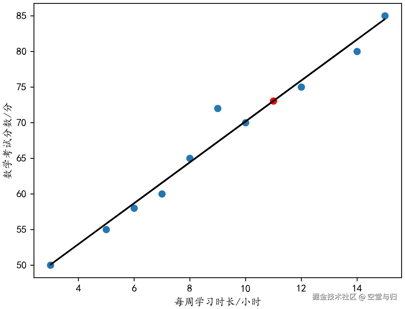
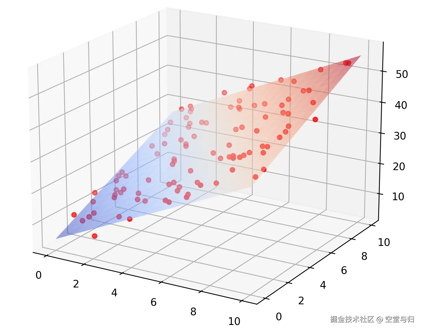
线性回归（Linear Regression）是建模变量之间线性关系的统计方法。它通过拟合一条直线（或高维空间的超平面），描述自变量（输入特征）与因变量（输出目标）之间的关联，核心目标是让预测值尽可能接近真实值。

核心公式 ： $y=w1x1+w2x2+...+wnxn+b\; y\; =\; w\_1x\_1\; +\; w\_2x\_2\; +\; ...\; +\; w\_nx\_n\; +\; b$ y=w1x1+w2x2+...+wnxn+b

• $wi\; w\_i$ wi：自变量的系数，表示每个特征对预测结果的影响程度
• $bb$ b：截距，所有特征为0时的基准值
• 通过估计这些参数，使模型预测值逼近真实值

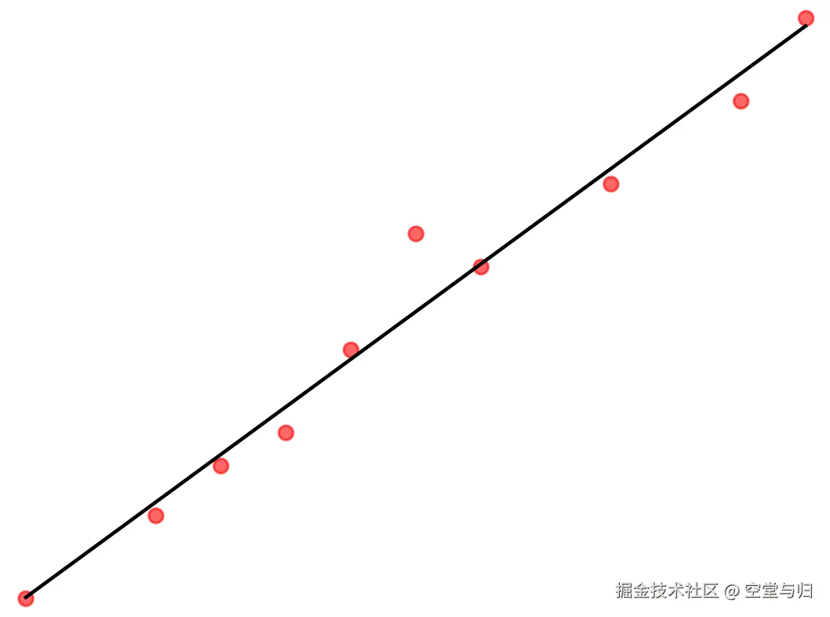
（上图：线性回归模型拟合数据点，直线为最优回归线，使所有数据点到直线的距离平方和最小）

1.2 一元 vs 多元线性回归

按照自变量的数量，线性回归分为两类：

• 一元线性回归 ：仅一个自变量，公式 $y=wx+by\; =\; wx\; +\; b$ y=wx+b。适合简单的单因素预测场景，比如"根据服务器CPU使用率预测响应时间"。
• 多元线性回归 ：包含多个自变量，公式 $y=w1x1+w2x2+...+wnxn+b\; y\; =\; w\_1x\_1\; +\; w\_2x\_2\; +\; ...\; +\; w\_nx\_n\; +\; b$ y=w1x1+w2x2+...+wnxn+b。实际项目中最常用，因为影响一个结果的因素往往不止一个。

from sklearn.linear_model import LinearRegression
import numpy as np

X = np.array([[10], [25], [40], [55], [70], [85], [15], [30], [45], [60]])
y = np.array([80, 120, 160, 200, 240, 280, 95, 135, 175, 215])

model = LinearRegression()
model.fit(X, y)

print(f"系数: {model.coef_}")
print(f"截距: {model.intercept_}")
cpu_usage = [[35]]
predicted_latency = model.predict(cpu_usage)
print(f"CPU 35% 时预测响应时间: {predicted_latency[0]:.1f}ms")

1.3 线性回归能用在哪些场景？

线性回归看似简单，却在实际工程中应用广泛：

• API性能预测：根据CPU、内存、网络请求量预测接口响应延迟
• 资源容量规划：基于历史用户增长数据预测服务器扩容需求
• 成本估算：根据广告投放渠道、时长、转化率预测获客成本
• SLA监控：根据系统负载指标预测服务可用性指标
• A/B测试分析：根据用户行为特征预测功能改版后的留存率

二、线性回归求解：从损失函数到最优解

2.1 损失函数：MSE与MAE怎么选？

要让模型精准，首先得定义"精准"的标准------这就是损失函数。损失函数衡量预测值与真实值的差距，我们的目标是最小化它。

均方误差（MSE） 是回归任务最常用的损失函数：

$MSE=1n\; \sum i=1n\; (yi-\; y^i\; )2\; MSE\; =\; \backslash frac\{1\}\{n\}\backslash sum\_\{i=1\}^n(y\_i\; -\; \backslash hat\{y\}\_i)^2$ MSE=n1∑i=1n(yi−y^i)2

MSE的核心特点：

• 对大误差敏感（平方放大效应），适合需要严惩大偏差的场景
• 是凸函数，有全局唯一最小值，便于求解
• 处处可导，便于梯度下降优化
• 当误差服从正态分布时，MSE等价于极大似然估计

平均绝对误差（MAE） 则对异常值更鲁棒：

$MAE=1n\; \sum i=1n\; \mid yi-\; y^i\; \mid \; MAE\; =\; \backslash frac\{1\}\{n\}\backslash sum\_\{i=1\}^n|y\_i\; -\; \backslash hat\{y\}\_i|$ MAE=n1∑i=1n∣yi−y^i∣

MAE的特点：对异常值不敏感，但对大误差惩罚较弱。适合数据中存在极端异常值的场景（如金融风险预测）。

选择建议：MSE用于模型训练的损失函数，MAE用于报告评估指标。

2.2 最小二乘法与解析解

基于MSE最小化来求解模型参数的方法称为最小二乘法。其几何意义是：找到一条直线（或超平面），使所有样本点到该直线的欧氏距离之和最小。

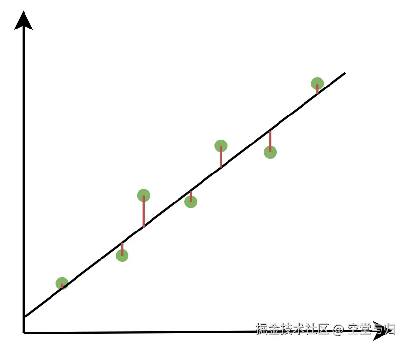
（上图：垂直线段表示每个数据点的残差（真实值-预测值），线性回归的目标是最小化所有残差的平方和）

对于一元线性回归，我们可以通过对损失函数求偏导并令其为0，直接得到解析解：

$w=\; \sum (xi-xˉ)(yi-yˉ)\; \sum (xi-xˉ)2\; w\; =\; \backslash frac\{\backslash sum(x\_i\; -\; \backslash bar\{x\})(y\_i\; -\; \backslash bar\{y\})\}\{\backslash sum(x\_i\; -\; \backslash bar\{x\})^2\}$ w=∑(xi−xˉ)2∑(xi−xˉ)(yi−yˉ)

$b=yˉ-wxˉ\; b\; =\; \backslash bar\{y\}\; -\; w\backslash bar\{x\}$ b=yˉ−wxˉ

def analytical_solution(X, y):
    """
    一元线性回归解析解
    直接通过数学公式计算最优参数，无需迭代
    """
    x_mean = np.mean(X)
    y_mean = np.mean(y)
    numerator = np.sum((X - x_mean) * (y - y_mean))
    denominator = np.sum((X - x_mean) ** 2)
    w = numerator / denominator
    b = y_mean - w * x_mean
    return w, b

X = np.array([10, 25, 40, 55, 70, 85, 15, 30, 45, 60])
y = np.array([80, 120, 160, 200, 240, 280, 95, 135, 175, 215])

w, b = analytical_solution(X, y)
print(f"解析解: w={w:.4f}, b={b:.4f}")
print(f"预测 CPU 35% 时的延迟: {w * 35 + b:.1f}ms")

2.3 正规方程法：直接算出最优参数

对于多元线性回归，解析解推广为正规方程（Normal Equation），通过矩阵运算直接求解：

$\theta =(XTX)-1XTy\backslash theta\; =\; (X^TX)^\{-1\}X^Ty$ θ=(XTX)−1XTy

其中：

• $XX$ X：包含全1列的特征矩阵（ $n\times (d+1)n\; \backslash times\; (d+1)$ n×(d+1) 维）
• $yy$ y：因变量向量（ $nn$ n 维）
• $\theta \backslash theta$ θ：参数向量（包含截距项）

正规方程法 vs 梯度下降：

对比项	正规方程法	梯度下降法
计算方式	矩阵运算直接求解	迭代逼近
时间复杂度	$O(nd2)O(nd^2)$ O(nd2)，d为特征数	迭代轮数 × O(nd)
适用场景	特征数量较少（d < 1000）	大数据集、特征多
超参数	无（无需调学习率）	需要调学习率
优缺点	简单直接，但需计算逆矩阵	适用于大规模数据

from sklearn.linear_model import LinearRegression
from sklearn.preprocessing import StandardScaler

X_multi = np.array([
    [10, 50, 200],
    [25, 60, 350],
    [40, 70, 500],
    [55, 80, 650],
    [70, 90, 800],
    [85, 95, 950],
    [15, 55, 250],
    [30, 65, 400],
])
y_multi = np.array([80, 120, 160, 200, 240, 280, 95, 135])

scaler = StandardScaler()
X_scaled = scaler.fit_transform(X_multi)

model_normal = LinearRegression(fit_intercept=True)
model_normal.fit(X_scaled, y_multi)

print(f"正规方程法系数: {model_normal.coef_}")
print(f"正规方程法偏置: {model_normal.intercept_:.4f}")

new_server = np.array([[35, 75, 600]])
new_server_scaled = scaler.transform(new_server)
prediction = model_normal.predict(new_server_scaled)
print(f"预测响应时间: {prediction[0]:.1f}ms")

2.4 梯度下降法：迭代逼近最优解

当特征数量很大时，正规方程中 $(XTX)-1(X^TX)^\{-1\}$ (XTX)−1 的计算成本急剧增加，此时梯度下降法更为适用。

梯度下降的核心思想：沿着损失函数的负梯度方向（下降最快的方向），逐步调整参数，直到收敛到最小值。

更新公式 ： $\theta t+1\; =\theta t-\alpha \cdot \nabla J(\theta t)\; \backslash theta\_\{t+1\}\; =\; \backslash theta\_t\; -\; \backslash alpha\; \backslash cdot\; \backslash nabla\; J(\backslash theta\_t)$ θt+1=θt−α⋅∇J(θt)

• $\alpha \backslash alpha$ α：学习率（Learning Rate），控制每步移动的距离
• $\nabla J(\theta )\backslash nabla\; J(\backslash theta)$ ∇J(θ)：损失函数对参数的梯度（偏导数向量）

（上图：梯度下降在3D曲面上的迭代路径，从初始点沿负梯度方向逐步逼近损失函数最小值点）

import numpy as np

def gradient_descent_demo():
    """
    梯度下降法求解线性回归
    目标函数: J(w, b) = (1/n) * Σ(y_i - (w*x_i + b))²
    """
    X = np.array([10, 25, 40, 55, 70, 85, 15, 30, 45, 60])
    y = np.array([80, 120, 160, 200, 240, 280, 95, 135, 175, 215])
    n = len(X)

    X_bias = np.column_stack([np.ones(n), X])

    theta = np.array([1.0, 1.0])
    alpha = 0.0001
    max_epochs = 10000
    tolerance = 1e-8

    for epoch in range(1, max_epochs + 1):
        predictions = X_bias @ theta
        errors = predictions - y
        gradient = (2 / n) * (X_bias.T @ errors)
        theta_new = theta - alpha * gradient

        if np.linalg.norm(theta_new - theta) < tolerance:
            theta = theta_new
            print(f"收敛于第 {epoch} 轮")
            break

        theta = theta_new

    print(f"梯度下降结果: b={theta[0]:.4f}, w={theta[1]:.4f}")
    print(f"预测 CPU 35% 时延迟: {theta[1] * 35 + theta[0]:.1f}ms")

gradient_descent_demo()

2.5 学习率怎么选？太大太小都不行

学习率是梯度下降中最关键的超参数：

• 学习率太大：可能跳过最优解，甚至在最优点附近震荡或发散
• 学习率太小：收敛速度慢，训练效率低下
• 自适应学习率：使用Adam、Adagrad等优化器自动调整，实践中最常用

（上图：左图学习率过大导致发散，中图学习率适中收敛良好，右图学习率过小收敛缓慢）

梯度下降的三种变体：

类型	描述	适用场景
批量梯度下降（BGD）	每次用全量数据计算梯度	小数据集、需要稳定收敛
随机梯度下降（SGD）	每次随机选1个样本	大数据集、在线学习
小批量梯度下降（MBGD）	每次用一小批样本	实践中最常用，平衡速度与稳定

from sklearn.linear_model import SGDRegressor
from sklearn.preprocessing import StandardScaler

X = np.array([[10, 50], [25, 60], [40, 70], [55, 80], [70, 90], [85, 95]])
y = np.array([80, 120, 160, 200, 240, 280])

scaler = StandardScaler()
X_scaled = scaler.fit_transform(X)

model_sgd = SGDRegressor(
    loss="squared_error",
    learning_rate="constant",
    eta0=0.01,
    max_iter=1000,
    tol=1e-8,
    random_state=42
)
model_sgd.fit(X_scaled, y)

print(f"SGD系数: {model_sgd.coef_}")
print(f"SGD偏置: {model_sgd.intercept_}")

三、实战：用线性回归预测API响应时间

下面用一个完整的实战案例串起前面的知识点。假设我们需要根据服务器的CPU使用率和内存占用率，预测API的响应时间，用于实时监控和自动扩缩容决策。

import pandas as pd
import numpy as np
from sklearn.model_selection import train_test_split
from sklearn.preprocessing import StandardScaler
from sklearn.linear_model import LinearRegression, SGDRegressor
from sklearn.metrics import mean_squared_error, mean_absolute_error, r2_score

np.random.seed(42)
n_samples = 200

data = {
    "cpu_usage": np.random.uniform(5, 95, n_samples),
    "memory_usage": np.random.uniform(20, 90, n_samples),
    "request_count": np.random.uniform(100, 5000, n_samples),
}

base_latency = (data["cpu_usage"] * 2.5 +
                data["memory_usage"] * 0.8 +
                data["request_count"] * 0.015)
noise = np.random.normal(0, 15, n_samples)
data["latency"] = base_latency + noise

df = pd.DataFrame(data)

X = df[["cpu_usage", "memory_usage", "request_count"]]
y = df["latency"]

x_train, x_test, y_train, y_test = train_test_split(
    X, y, test_size=0.3, random_state=42
)

scaler = StandardScaler()
x_train_scaled = scaler.fit_transform(x_train)
x_test_scaled = scaler.transform(x_test)

lr_model = LinearRegression()
lr_model.fit(x_train_scaled, y_train)

sgd_model = SGDRegressor(max_iter=5000, tol=1e-8, random_state=42)
sgd_model.fit(x_train_scaled, y_train)

lr_pred = lr_model.predict(x_test_scaled)
sgd_pred = sgd_model.predict(x_test_scaled)

print("=" * 50)
print("正规方程法 vs 随机梯度下降法 对比")
print("=" * 50)
print(f"正规方程法 MSE: {mean_squared_error(y_test, lr_pred):.2f}")
print(f"正规方程法 MAE: {mean_absolute_error(y_test, lr_pred):.2f}")
print(f"正规方程法 R²:  {r2_score(y_test, lr_pred):.4f}")
print()
print(f"随机梯度下降 MSE: {mean_squared_error(y_test, sgd_pred):.2f}")
print(f"随机梯度下降 MAE: {mean_absolute_error(y_test, sgd_pred):.2f}")
print(f"随机梯度下降 R²:  {r2_score(y_test, sgd_pred):.4f}")
print()
print(f"正规方程法系数: CPU={lr_model.coef_[0]:.2f}, 内存={lr_model.coef_[1]:.2f}, 请求量={lr_model.coef_[2]:.4f}")
print(f"正规方程法偏置: {lr_model.intercept_:.2f}")

new_metrics = pd.DataFrame({
    "cpu_usage": [45, 75, 90],
    "memory_usage": [60, 80, 95],
    "request_count": [2000, 3500, 4800],
})
new_metrics_scaled = scaler.transform(new_metrics)
predictions = lr_model.predict(new_metrics_scaled)
print()
print("实时预测示例:")
for i, (_, row) in enumerate(new_metrics.iterrows()):
    print(f"  CPU={row['cpu_usage']}%, 内存={row['memory_usage']}%, 请求={row['request_count']:.0f} → 预测延迟={predictions[i]:.1f}ms")

关键发现：正规方程法和梯度下降法得到的结果非常接近，因为它们优化的是同一个损失函数。特征系数告诉我们，CPU使用率对响应时间的影响最大（系数最大），这符合直觉。

常见问题

为什么线性回归预测不准？排查这几个原因

很多同学反馈线性回归预测效果差，其实问题往往不在模型本身，而在数据和预处理上。常见原因包括：特征与目标变量之间不是线性关系（此时应使用非线性模型或对特征做多项式变换）、特征之间存在多重共线性（如CPU和内存使用率高度相关，可以用PCA降维或正则化）、数据中存在大量异常值（可以用MAE替代MSE，或先做异常值处理）。

什么时候用正规方程，什么时候用梯度下降？

这个问题的核心是数据规模。如果特征数量较少（通常d < 1000）且数据集不大，正规方程法是更好的选择------无需调学习率，直接得到精确解。但当特征数量庞大或数据集很大时，正规方程需要计算 $(XTX)-1(X^TX)^\{-1\}$ (XTX)−1，复杂度为 $O(nd2)O(nd^2)$ O(nd2)，此时梯度下降更高效。实践中，scikit-learn的LinearRegression默认使用正规方程，SGDRegressor使用梯度下降，两者在数据规模适中时结果差异很小。

MSE和MAE到底选哪个？

MSE和MAE各有优势。MSE对大误差更敏感（平方放大），如果你希望严厉惩罚预测严重偏差的情况（如故障预警、安全监控），MSE是更好的选择。MAE对异常值更鲁棒，适合数据中可能存在极端值的场景（如金融预测、用户行为分析）。实际工作中的黄金组合是：用MSE作为训练损失函数（便于梯度下降优化），用MAE作为报告指标（更直观、对异常值不敏感）。

学习率调了很多次还是不收敛？

学习率调优是梯度下降中最头疼的问题。如果你试过多个固定学习率都不行，不妨试试自适应优化器（Adam、Adagrad），它们会在训练过程中自动调整每个参数的学习率。另一个常见陷阱是特征没有做标准化 ------如果不同特征的量级差异很大（如CPU百分比0-100 vs 请求量100-5000），损失函数会变成狭长的峡谷形状，导致梯度下降在某些方向上震荡。先标准化特征，再调学习率，往往能解决大部分收敛问题。

和 AI 大模型开发的关系

场景一：大模型API调用成本预测

在AI应用中，我们需要预测大模型API的调用成本（如Token消耗、费用），以便做预算规划和自动扩缩容。线性回归可以基于历史调用数据快速建模：

class LLMcostPredictor:
    def __init__(self):
        self.model = LinearRegression()
        self.scaler = StandardScaler()
        self.is_fitted = False

    def fit(self, historical_data):
        """
        基于历史调用数据训练成本预测模型
        historical_data: DataFrame包含 token_count, prompt_length, response_length, cost
        """
        features = ["token_count", "prompt_length", "response_length"]
        X = historical_data[features].values
        y = historical_data["cost"].values

        X_scaled = self.scaler.fit_transform(X)
        self.model.fit(X_scaled, y)
        self.is_fitted = True

        print(f"成本模型系数: {dict(zip(features, self.model.coef_))}")
        print(f"基准成本: {self.model.intercept_:.4f}")

    def predict_cost(self, token_count, prompt_length, response_length):
        """
        预测API调用成本
        """
        if not self.is_fitted:
            raise ValueError("请先使用 fit() 训练模型")

        features = np.array([[token_count, prompt_length, response_length]])
        features_scaled = self.scaler.transform(features)
        predicted_cost = self.model.predict(features_scaled)[0]
        return max(0, predicted_cost)

training_data = pd.DataFrame({
    "token_count": [1000, 2500, 5000, 8000, 12000, 15000],
    "prompt_length": [100, 250, 500, 800, 1200, 1500],
    "response_length": [200, 500, 1000, 1500, 2500, 3000],
    "cost": [0.002, 0.005, 0.010, 0.016, 0.024, 0.030],
})

predictor = LLMcostPredictor()
predictor.fit(training_data)

cost = predictor.predict_cost(
    token_count=6000,
    prompt_length=600,
    response_length=1200
)
print(f"预测成本: ${cost:.4f}")

场景二：Agent任务执行延迟预测

在Agent系统中，任务调度需要预估每个任务的执行时间，以便合理分配资源和设置超时。线性回归可以基于任务特征（子任务数量、工具调用次数、数据量大小）预测执行延迟：

class AgentTaskLatencyEstimator:
    def __init__(self):
        self.model = SGDRegressor(max_iter=1000, tol=1e-5)
        self.scaler = StandardScaler()

    def train(self, task_features, latencies):
        """
        训练延迟预测模型
        task_features: [子任务数, 工具调用次数, 数据量(MB), 模型调用次数]
        latencies: 实际执行延迟(秒)
        """
        X_scaled = self.scaler.fit_transform(task_features)
        self.model.fit(X_scaled, latencies)

    def estimate_timeout(self, subtasks, tool_calls, data_size, llm_calls, safety_factor=1.5):
        """
        估算任务超时阈值（预测值 × 安全系数）
        """
        features = np.array([[subtasks, tool_calls, data_size, llm_calls]])
        features_scaled = self.scaler.transform(features)
        predicted = self.model.predict(features_scaled)[0]
        return predicted * safety_factor

task_data = np.array([
    [3, 5, 2.5, 2],
    [5, 8, 5.0, 4],
    [2, 3, 1.0, 1],
    [8, 12, 10.0, 6],
    [4, 6, 3.0, 3],
])
latencies = np.array([12, 25, 8, 45, 18])

estimator = AgentTaskLatencyEstimator()
estimator.train(task_data, latencies)

timeout = estimator.estimate_timeout(
    subtasks=6,
    tool_calls=10,
    data_size=8.0,
    llm_calls=5
)
print(f"预计执行时间: {timeout / 1.5:.1f}s, 超时阈值: {timeout:.1f}s")

场景三：RAG检索质量预测

在RAG系统中，我们可以基于文档的特征（长度、关键词密度、嵌入向量范数）预测检索质量（如相关性得分），从而优化检索策略：

class RAGQualityPredictor:
    def __init__(self):
        self.model = LinearRegression()
        self.scaler = StandardScaler()

    def build_training_data(self, documents, relevance_scores):
        """
        构建训练数据：从文档中提取特征
        """
        features = []
        for doc in documents:
            feature_vector = [
                len(doc.split()),
                len(set(doc.lower().split())),
                doc.count("important") + doc.count("key") + doc.count("critical"),
                len(doc) / max(1, len(doc.split())),
            ]
            features.append(feature_vector)
        return np.array(features), np.array(relevance_scores)

    def train(self, documents, scores):
        X, y = self.build_training_data(documents, scores)
        X_scaled = self.scaler.fit_transform(X)
        self.model.fit(X_scaled, y)
        print(f"特征重要性: 长度={self.model.coef_[0]:.3f}, "
              f"词汇丰富度={self.model.coef_[1]:.3f}, "
              f"关键词密度={self.model.coef_[2]:.3f}")

    def predict_quality(self, documents):
        X, _ = self.build_training_data(documents, [0] * len(documents))
        X_scaled = self.scaler.transform(X)
        return self.model.predict(X_scaled)

docs = [
    "This is a very important document with key information about critical systems",
    "Short text",
    "Critical important key data about machine learning models and their applications",
]
scores = [0.85, 0.30, 0.92]

predictor = RAGQualityPredictor()
predictor.train(docs, scores)

new_docs = [
    "Important critical key data about neural network architectures",
]
quality = predictor.predict_quality(new_docs)
print(f"预测检索质量得分: {quality[0]:.3f}")

总结

线性回归虽然简单，但它是理解机器学习核心思想的最佳入门模型。本文从三个层面系统讲解了线性回归：

模型层面：理解线性回归的本质是拟合自变量与因变量之间的线性关系，掌握一元与多元线性回归的区别与联系。

求解层面：对比了三种主流求解方法------最小二乘法（解析解）、正规方程法（矩阵求解）和梯度下降法（迭代优化），明确了各自的适用场景。重点理解MSE作为损失函数的意义，以及学习率对梯度下降收敛的影响。

工程层面：通过API响应时间预测的完整实战，串联了数据预处理、特征工程、模型训练、评估和部署的全流程。三个AI大模型开发场景（成本预测、任务调度、RAG质量评估）展示了线性回归在AI系统设计中的实际价值。

掌握线性回归，不仅能解决大量实际的预测问题，更为后续学习逻辑回归、正则化、乃至神经网络打下坚实基础。

---

#线性回归 #机器学习 #数据预测 #梯度下降 #正规方程