Python入门到高级（知识点七）

📚 Python入门到高级（知识点七）

---

💡 关键知识点

RFM客户价值分析完整案例

一、什么是RFM模型

RFM模型是衡量客户价值的经典方法，通过三个维度评估客户：

维度	全称	含义	分值越高代表
R	Recency（最近一次消费）	客户最近一次购买时间距今多久	越近越好（天数越少）
F	Frequency（消费频率）	客户在一定时间内购买次数	购买越频繁越好
M	Monetary（消费金额）	客户一定时间内的消费总金额	消费越多越好

---

二、完整代码实现

# 1. 导包
import numpy as np
import pandas as pd
import matplotlib.pyplot as plt

# 解决个别版本show()无法展示图的问题
import matplotlib
matplotlib.use('TkAgg')

# 解决中文乱码问题
plt.rcParams['font.sans-serif'] = ['SimHei']

# 额外安装: pip install openpyxl（用于读取.xlsx文件）

# 2. 加载数据
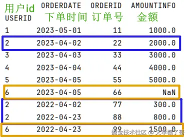
df = pd.read_excel("data/sales_test.xlsx", index_col='USERID')
print(df.shape)  # (9, 3)

# 3. 数据预处理
# 删除全部为空的行
sale_data = df.dropna(how='all')
print(sale_data.shape)
print(sale_data.columns)

---

三、计算R、F、M三个维度

3.1 计算F（购买频率）------ 统计每个用户的订单数

# 按用户ID分组，统计每个用户的订单数量
F_data = sale_data.groupby(sale_data.index)['ORDERID'].count()
# 示例输出（假设数据）：
# USERID
# 1001    3
# 1002    1
# 1003    2
# Name: ORDERID, dtype: int64

3.2 计算M（消费金额）------ 每个用户的订单总金额

# 按用户ID分组，对AMOUNTINFO列求和
M_data = sale_data.groupby(sale_data.index)['AMOUNTINFO'].sum()
# 示例输出（假设数据）：
# USERID
# 1001    1800.0
# 1002     500.0
# 1003    1200.0
# Name: AMOUNTINFO, dtype: float64

3.3 计算R（最近购买时间）------ 每个用户最近一次下单日期

# 按用户ID分组，取ORDERDATE的最大值（最近的日期）
R_data = sale_data.groupby(sale_data.index)['ORDERDATE'].max()
# 示例输出（假设数据）：
# USERID
# 1001    2022-03-20
# 1002    2022-01-15
# 1003    2022-02-28
# Name: ORDERDATE, dtype: datetime64[ns]

---

四、计算R、F、M的分数（1-5分）

4.1 F分数和M分数

# F_score: 用pd.cut将F_data分成5个等级，1最低，5最高
F_score = pd.cut(F_data, 5, labels=[1, 2, 3, 4, 5])

# M_score: 同理，按金额分成5个等级
M_score = pd.cut(M_data, 5, labels=[1, 2, 3, 4, 5])

pd.cut() 工作原理：

数据范围	标签
最小值 ~ 20%分位	1
20% ~ 40%分位	2
40% ~ 60%分位	3
60% ~ 80%分位	4
80% ~ 最大值	5

4.2 R分数（注意：天数越少分数越高）

# 设置一个基准日期（比所有订单日期都晚）
base_date = pd.to_datetime("2022-04-01")

# 计算每个用户最近购买日距离基准日期的天数
R_days = (R_data - base_date).dt.days
# 示例：2022-03-20距离2022-04-01 = -12天（过去12天）

# R分数：距离越近（天数越大？负数绝对值越小）分数越高
R_score = pd.cut(R_days, 5, labels=[1, 2, 3, 4, 5])

R分数理解：

最近购买日期	距基准日天数	分数
2022-03-28	-4	5（最近）
2022-03-15	-17	4
2022-02-20	-40	3
2022-01-10	-81	2
2021-12-01	-121	1（最远）

---

五、合并R、F、M分数

# 将三个分数合并成一个DataFrame
rfm_list = [R_score, F_score, M_score]
rfm_cols = ['r_score', 'f_score', 'm_score']

# .transpose() 将3行×N列 转置为 N行×3列
rfm_df = pd.DataFrame(
    np.array(rfm_list).transpose(),
    dtype=np.int32,
    columns=rfm_cols,
    index=R_data.index
)
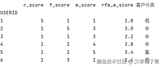
print(rfm_df)

转置前后对比：

转置前（3行×N列）：
        USERID_1  USERID_2  USERID_3  ...
r_score    5         4          3
f_score    3         1          2
m_score    5         2          4

转置后（N行×3列）：
         r_score  f_score  m_score
USERID_1    5        3        5
USERID_2    4        1        2
USERID_3    3        2        4

---

六、计算加权综合得分

# 商家根据业务需求设置权重
# 例如：交易时间20% + 交易次数20% + 交易金额60%
rfm_df['rfm_w_score'] = (
    rfm_df['r_score'] * 0.2 +
    rfm_df['f_score'] * 0.2 +
    rfm_df['m_score'] * 0.6
)

权重分配示例：

业务场景	R权重	F权重	M权重	说明
注重客单价	10%	10%	80%	金额最重要
注重活跃度	50%	30%	20%	最近购买最重要
均衡型	33%	33%	34%	三者均衡

---

七、客户分层与可视化

# 7.1 根据综合得分划分客户等级
bins = [0, 2, 3, 5]  # 区间：[0,2)、[2,3)、[3,5]
labels = ['低', '中', '高']
rfm_df['客户分类'] = pd.cut(rfm_df['rfm_w_score'], bins=bins, labels=labels)
print(rfm_df)

# 7.2 绘制柱状图
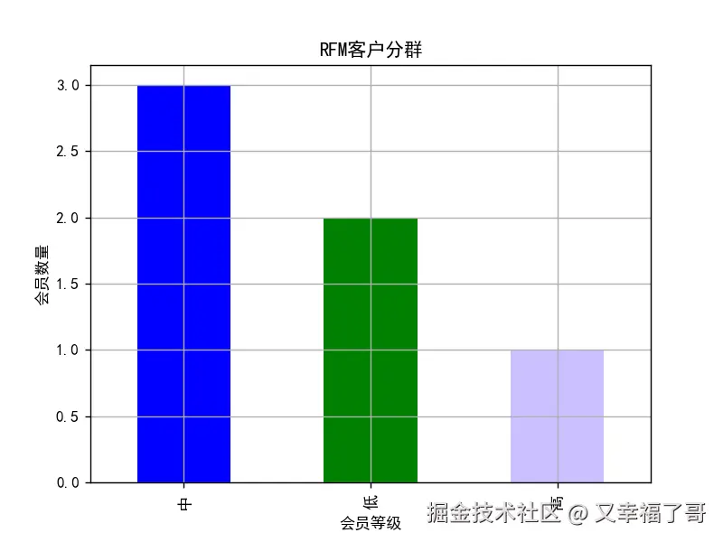
rfm_df['客户分类'].value_counts().plot(
    kind='bar',
    color=['red', 'green', 'pink']
)
plt.title('RFM客户分群')
plt.xlabel('会员等级')
plt.ylabel('会员数量')
plt.grid()
plt.show()

# 7.3 保存结果到本地
rfm_df.to_csv('data/rfm_score.txt')

---

八、RFM应用场景总结

客户等级	特征	营销策略
高价值	R低（最近购买）、F高（频繁）、M高（金额大）	VIP维护、专属优惠
中价值	部分维度表现中等	持续培养、提升消费
低价值	R高（很久没买）、F低（不活跃）、M低（消费少）	促销唤醒、放弃维护

---

九、完整代码汇总

# 1. 导包
import numpy as np
import pandas as pd
import matplotlib.pyplot as plt
import matplotlib
matplotlib.use('TkAgg')
plt.rcParams['font.sans-serif'] = ['SimHei']

# 2. 加载数据
df = pd.read_excel("data/sales_test.xlsx", index_col='USERID')

# 3. 数据预处理（删除全空行）
sale_data = df.dropna(how='all')

# 4. 计算RFM三值
F_data = sale_data.groupby(sale_data.index)['ORDERID'].count()
M_data = sale_data.groupby(sale_data.index)['AMOUNTINFO'].sum()
R_data = sale_data.groupby(sale_data.index)['ORDERDATE'].max()

# 5. 计算RFM分数
F_score = pd.cut(F_data, 5, labels=[1, 2, 3, 4, 5])
M_score = pd.cut(M_data, 5, labels=[1, 2, 3, 4, 5])
base_date = pd.to_datetime("2022-04-01")
R_days = (R_data - base_date).dt.days
R_score = pd.cut(R_days, 5, labels=[1, 2, 3, 4, 5])

# 6. 合并分数
rfm_df = pd.DataFrame(
    np.array([R_score, F_score, M_score]).transpose(),
    dtype=np.int32,
    columns=['r_score', 'f_score', 'm_score'],
    index=R_data.index
)

# 7. 加权得分
rfm_df['rfm_w_score'] = (
    rfm_df['r_score'] * 0.2 +
    rfm_df['f_score'] * 0.2 +
    rfm_df['m_score'] * 0.6
)

# 8. 客户分层
rfm_df['客户分类'] = pd.cut(rfm_df['rfm_w_score'], bins=[0, 2, 3, 5], labels=['低', '中', '高'])

# 9. 可视化
rfm_df['客户分类'].value_counts().plot(kind='bar', color=['red', 'green', 'pink'])
plt.title('RFM客户分群')
plt.xlabel('会员等级')
plt.ylabel('会员数量')
plt.grid()
plt.show()

# 10. 保存结果
rfm_df.to_csv('data/rfm_score.txt')