尼泊尔河流流量:天气驱动的预测与高流量风险
本笔记本使用一个日频数据集,涵盖 2023-01-01 至 2026-08-31 期间 尼泊尔的 10 个河流测站 。每一行对应一个站点-日,将天气变量(降水量、降雨量、土壤湿度、温度、湿度、风速)与当天的实测河流流量(river_discharge_m3s)结合在一起。
本笔记本有两个相互关联的目标:
- 理解天气与河流流量之间的关系:季节性模式、站点之间的差异,以及今天的降雨如何在随后几天的流量中体现(降雨-流量滞后)。
- 预测 关于明天 的两件事,且仅使用截至今天 可获得的信息:
- 次日流量(回归):实际的 m³/s 数值。
- 次日高流量状态(分类) :明天的流量对该站点而言在统计上是否异常(高于其自身的第 95 百分位数),在此用作统计意义上的洪水风险代理指标,而非官方洪水预警。
下文中的所有数字、表格和图表均直接基于上传的 V2 数据集计算得出。没有凭空捏造或假设任何分数、阈值或结论------凡笔记本陈述某个结果之处,其上方的单元格都会计算出该结果。
**关于范围的说明:*该数据集不包含官方 DHM 洪水预警标签,没有洪水影响/暴露数据,也没有河网汇流演算。因此,本笔记本中的"洪水风险"始终指"相对于该站点自身历史、容量而言统计上偏高的流量状态"*,绝非可用于实际业务的洪水预报。
2. 数据集概览与数据质量
python
import numpy as np
import pandas as pd
import matplotlib.pyplot as plt
import matplotlib.dates as mdates
import seaborn as sns

import warnings
warnings.filterwarnings('ignore')

sns.set_style("whitegrid")
pd.set_option("display.max_columns", None)
pd.set_option("display.width", 140)
plt.rcParams["figure.dpi"] = 100
RNG_SEED = 42

DATA_PATH = "/kaggle/input/datasets/tejal5kunjir/nepal-flood-and-weather-dataset-2023-2026/CORRECTED_2023_2026_NEPAL_FLOOD_WEATHER_KAGGLE.csv"
import os

df = pd.read_csv(DATA_PATH)
df.columns = [c.strip() for c in df.columns]
df["date"] = pd.to_datetime(df["date"])
df = df.sort_values(["location", "date"]).reset_index(drop=True)
df["year"] = df["date"].dt.year
df["month"] = df["date"].dt.month

print(f"Rows: {df.shape[0]}, Columns: {df.shape[1]}")
print(f"Date range: {df['date'].min().date()} to {df['date'].max().date()}")
print(f"Stations: {df['location'].nunique()}")


print("rain_mm == precipitation_mm:", (df["rain_mm"] == df["precipitation_mm"]).mean())
text
Rows: 13390, Columns: 21
Date range: 2023-01-01 to 2026-08-31
Stations: 10
rain_mm == precipitation_mm: 0.9830470500373413
python
#first 5 rows
df.head()
text
date   location        river  basin  dhm_station   latitude  longitude  elevation_m  precipitation_mm  soil_moisture_0_100cm_m3m3  \
0 2023-01-01  Bahrabise  Bhote Koshi  Koshi        610.0  27.786773  85.899324         1870               0.0                       0.291
1 2023-01-02  Bahrabise  Bhote Koshi  Koshi        610.0  27.786773  85.899324         1870               0.0                       0.303
2 2023-01-03  Bahrabise  Bhote Koshi  Koshi        610.0  27.786773  85.899324         1870               0.0                       0.306
3 2023-01-04  Bahrabise  Bhote Koshi  Koshi        610.0  27.786773  85.899324         1870               0.0                       0.308
4 2023-01-05  Bahrabise  Bhote Koshi  Koshi        610.0  27.786773  85.899324         1870               0.0                       0.308

   rain_mm  temperature_mean_c  dew_point_mean_c  precipitation_hours  relative_humidity_mean_pct  wind_speed_max_kmh  wind_gusts_max_kmh  \
0      0.0                12.3               6.8                    0                          71                 7.8                24.1
1      0.0                11.3               6.1                    0                          73                 7.3                25.2
2      0.0                10.6               3.6                    0                          65                 7.9                24.1
3      0.0                10.0               2.2                    0                          61                 8.0                22.3
4      0.0                11.3               1.9                    0                          55                 5.9                21.6

   wind_direction_dominant_deg  river_discharge_m3s  year  month
0                          106                 1.05  2023      1
1                           80                 1.05  2023      1
2                           89                 1.01  2023      1
3                           77                 0.99  2023      1
4                           67                 0.97  2023      1
python
#last 5 rows
df.tail()
text
date     location        river     basin  dhm_station   latitude  longitude  elevation_m  precipitation_mm  \
13385 2026-08-27  Rasuwagadhi  Bhote Koshi  Narayani       446.22  28.271297  85.377649         1749               2.9
13386 2026-08-28  Rasuwagadhi  Bhote Koshi  Narayani       446.22  28.271297  85.377649         1749               4.1
13387 2026-08-29  Rasuwagadhi  Bhote Koshi  Narayani       446.22  28.271297  85.377649         1749              25.6
13388 2026-08-30  Rasuwagadhi  Bhote Koshi  Narayani       446.22  28.271297  85.377649         1749               4.4
13389 2026-08-31  Rasuwagadhi  Bhote Koshi  Narayani       446.22  28.271297  85.377649         1749               5.5

       soil_moisture_0_100cm_m3m3  rain_mm  temperature_mean_c  dew_point_mean_c  precipitation_hours  relative_humidity_mean_pct  \
13385                       0.410      2.9                24.3              20.9                    7                          82
13386                       0.408      4.1                24.5              20.7                   20                          80
13387                       0.409     25.6                24.0              21.6                   24                          87
13388                       0.411      4.4                24.3              20.6                   16                          81
13389                       0.411      5.5                23.9              20.6                   18                          82

       wind_speed_max_kmh  wind_gusts_max_kmh  wind_direction_dominant_deg  river_discharge_m3s  year  month
13385                 6.7                40.0                          241                 4.04  2026      8
13386                 7.0                40.3                          229                 3.58  2026      8
13387                 4.2                31.3                          244                 3.47  2026      8
13388                 7.0                37.8                          236                 3.73  2026      8
13389                 4.4                33.5                          246                 3.60  2026      8
python
#datatype of each column
df.dtypes
text
date                           datetime64[ns]
location                               object
river                                  object
basin                                  object
dhm_station                           float64
latitude                              float64
longitude                             float64
elevation_m                             int64
precipitation_mm                      float64
soil_moisture_0_100cm_m3m3            float64
rain_mm                               float64
temperature_mean_c                    float64
dew_point_mean_c                      float64
precipitation_hours                     int64
relative_humidity_mean_pct              int64
wind_speed_max_kmh                    float64
wind_gusts_max_kmh                    float64
wind_direction_dominant_deg             int64
river_discharge_m3s                   float64
year                                    int32
month                                   int32
dtype: object
python
#quality check
quality = pd.DataFrame({
    "rows_per_station": df.groupby("location").size(),
    "date_min": df.groupby("location")["date"].min().dt.date,
    "date_max": df.groupby("location")["date"].max().dt.date,
    "null_values": df.groupby("location").apply(lambda g: g.isnull().sum().sum()),
})
quality["expected_days"] = (pd.to_datetime(quality["date_max"]) - pd.to_datetime(quality["date_min"])).dt.days + 1
quality["complete"] = quality["rows_per_station"] == quality["expected_days"]
quality
text
rows_per_station    date_min    date_max  null_values  expected_days  complete
location
Bahrabise                        1339  2023-01-01  2026-08-31            0           1339      True
Belsot                           1339  2023-01-01  2026-08-31            0           1339      True
Bhada Bridge                     1339  2023-01-01  2026-08-31            0           1339      True
Chameliya/Nayalbadi              1339  2023-01-01  2026-08-31            0           1339      True
Chatara                          1339  2023-01-01  2026-08-31            0           1339      True
Chisapani                        1339  2023-01-01  2026-08-31            0           1339      True
Devghat                          1339  2023-01-01  2026-08-31            0           1339      True
Khokana                          1339  2023-01-01  2026-08-31            0           1339      True
Kusum                            1339  2023-01-01  2026-08-31            0           1339      True
Rasuwagadhi                      1339  2023-01-01  2026-08-31            0           1339      True
python
#null & duplicate check
total_nulls = df.isnull().sum().sum()
dup_pairs = df.duplicated(subset=["date", "location"]).sum()
dup_rows = df.duplicated().sum()

print(f"Total null values in the whole dataset : {total_nulls}")
print(f"Duplicate (date, location) pairs       : {dup_pairs}")
print(f"Fully duplicate rows                    : {dup_rows}")

meta_cols   = ["location", "river", "basin", "dhm_station", "latitude", "longitude", "elevation_m"]
weather_cols = ["precipitation_mm", "rain_mm", "soil_moisture_0_100cm_m3m3", "temperature_mean_c",
                "dew_point_mean_c", "precipitation_hours", "relative_humidity_mean_pct",
                "wind_speed_max_kmh", "wind_gusts_max_kmh", "wind_direction_dominant_deg"]
target_col  = ["river_discharge_m3s"]

print("\nColumn groups")
print(f"  Station metadata ({len(meta_cols)}): {meta_cols}")
print(f"  Weather variables ({len(weather_cols)}): {weather_cols}")
print(f"  Target ({len(target_col)}): {target_col}")
text
Total null values in the whole dataset : 0
Duplicate (date, location) pairs       : 0
Fully duplicate rows                    : 0

Column groups
  Station metadata (7): ['location', 'river', 'basin', 'dhm_station', 'latitude', 'longitude', 'elevation_m']
  Weather variables (10): ['precipitation_mm', 'rain_mm', 'soil_moisture_0_100cm_m3m3', 'temperature_mean_c', 'dew_point_mean_c', 'precipitation_hours', 'relative_humidity_mean_pct', 'wind_speed_max_kmh', 'wind_gusts_max_kmh', 'wind_direction_dominant_deg']
  Target (1): ['river_discharge_m3s']
python
#river station wise data

stations = (df[["location", "river", "basin", "elevation_m"]]
            .drop_duplicates()
            .sort_values("location")
            .reset_index(drop=True))
stations
text
location        river            basin  elevation_m
0            Bahrabise  Bhote Koshi            Koshi         1870
1               Belsot       Kamala           Kamala          188
2         Bhada Bridge        Babai            Babai          157
3  Chameliya/Nayalbadi     Chamelia         Mahakali          685
4              Chatara   Saptakoshi            Koshi          153
5            Chisapani      Karnali          Karnali         2215
6              Devghat     Narayani  Narayani/Gandak          603
7              Khokana      Bagmati          Bagmati         1315
8                Kusum   West Rapti            Rapti          230
9          Rasuwagadhi  Bhote Koshi         Narayani         1749
3. 探索性数据分析
这 10 个站点位于截然不同的河流上,海拔也相差悬殊,因此我们预计它们的流量处于非常不同的量级(小山溪 vs. 大型干流河流)。下面的图表是经过挑选的,用于展示不同的内容,而不是重复同一种图表类型:
- 用对数刻度的箱线图/小提琴图展示各站点的整体流量分布(使极小和极大的河流可以在同一坐标轴上比较),
- 用折线图展示月平均流量(所有站点合并),作为对季节性的初步检验,
- 用散点图展示降水量与流量的关系,
- 用带透明度和趋势线的散点图展示湿度与降水量的关系,因为数据点超过 13,000 个,普通散点图只会呈现为一团实心色块。
python
#discharge distribution & discharge summary by station

order = df.groupby("location")["river_discharge_m3s"].median().sort_values(ascending=False).index

fig, ax = plt.subplots(figsize=(12, 8))

sns.boxplot(
    data=df,
    x="location",
    y="river_discharge_m3s",
    order=order,
    ax=ax

)

ax.set_yscale("log")
ax.set_ylabel("River discharge (m$^3$/s), log scale")
ax.set_xlabel("Station")
ax.set_title("Discharge distribution by station (log scale)")
ax.tick_params(axis="x", rotation=40)

plt.tight_layout()
plt.show()

print("Discharge summary by station (m3/s):")
df.groupby("location")["river_discharge_m3s"].describe()[
    ["min", "25%", "50%", "75%", "max"]
].loc[order]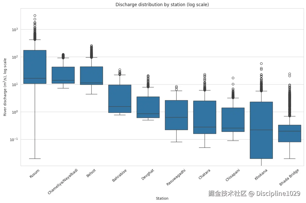
text
Discharge summary by station (m3/s):
text
min    25%    50%      75%      max
location
Kusum                0.02  10.67  16.86  176.215  3175.87
Chameliya/Nayalbadi  7.22  10.91  14.14   43.055   124.60
Belsot               4.41   9.74  11.42   43.820   255.45
Bahrabise            0.78   0.94   1.56    9.520    33.75
Devghat              0.50   0.61   0.86    3.560    20.78
Rasuwagadhi          0.08   0.22   0.63    2.625     8.33
Chatara              0.05   0.16   0.28    2.530    23.27
Chisapani            0.09   0.19   0.26    1.400    16.99
Khokana              0.00   0.02   0.22    2.310    57.61
Bhada Bridge         0.02   0.08   0.20    0.330    24.18
对数刻度显示各站点的流量水平差异很大。例如,Kusum 的流量通常在数百 m³/s,有时达到数千 m³/s,而 Bhada Bridge 和 Chisapani 通常低于 10 m³/s。这说明在预测流量时,站点身份非常重要,我们将在第 11 节中利用这一点。
python
#monthly discharge across all stations

monthly_all = df.groupby(df["date"].dt.to_period("M"))["river_discharge_m3s"].mean()
monthly_all.index = monthly_all.index.to_timestamp()

fig, ax = plt.subplots(figsize=(13, 4.5))
ax.plot(monthly_all.index, monthly_all.values, color="red", marker="o")
ax.set_title("Mean discharge across all stations, by month (2023-01 to 2026-08)")
ax.set_ylabel("Mean river discharge (m$^3$/s)")
ax.set_xlabel("Month")
ax.xaxis.set_major_locator(mdates.MonthLocator(interval=4))
ax.xaxis.set_major_formatter(mdates.DateFormatter("%Y-%m"))
plt.xticks(rotation=45)
plt.tight_layout()
plt.show()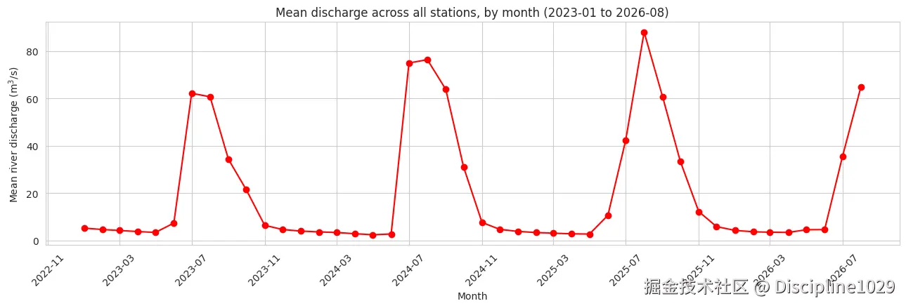
即使取全部十个站点的平均值,我们也能看到每年季风月份流量明显上升。然而,各站点的流量水平差异很大,因此平均值受流量较大的河流影响显著。第 4 节将分别考察每个站点,以更好地理解它们的季节性模式。
python
fig, ax = plt.subplots(figsize=(7, 6))
sample = df.sample(n=min(6000, len(df)), random_state=RNG_SEED)
ax.scatter(sample["precipitation_mm"], sample["river_discharge_m3s"], s=8, alpha=0.25, color="slateblue")
ax.set_yscale("log")
ax.set_xlabel("Precipitation (mm)")
ax.set_ylabel("River discharge (m$^3$/s), log scale")
ax.set_title("Precipitation vs. discharge (same-day, all stations)")
plt.tight_layout()
plt.show()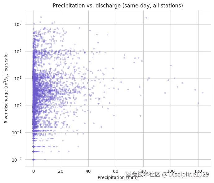
当日降雨量与流量之间呈现微弱的正相关,但数据点相当分散。相同的降雨量在不同站点、不同土壤条件以及不同前期降雨的情况下,可能导致截然不同的流量水平。这就是我们在第 5 节中考察不同时间滞后降雨量的原因。
python
fig, ax = plt.subplots(figsize=(7, 6))
x = df["relative_humidity_mean_pct"].values
y = df["precipitation_mm"].values
ax.scatter(x, y, s=6, alpha=0.12, color="green")

coeffs = np.polyfit(x, y, deg=1)
xs = np.linspace(x.min(), x.max(), 100)
ax.plot(xs, np.polyval(coeffs, xs), color="red", linewidth=2,
        label=f"trend: precip = {coeffs[0]:.2f}*humidity + {coeffs[1]:.2f}")
ax.set_xlabel("Relative humidity (mean, %)")
ax.set_ylabel("Precipitation (mm)")
ax.set_title("Humidity vs. precipitation (all stations, all days)")
ax.legend()
plt.tight_layout()
plt.show()

print("Correlation (humidity, precipitation):", round(np.corrcoef(x, y)[0, 1], 3))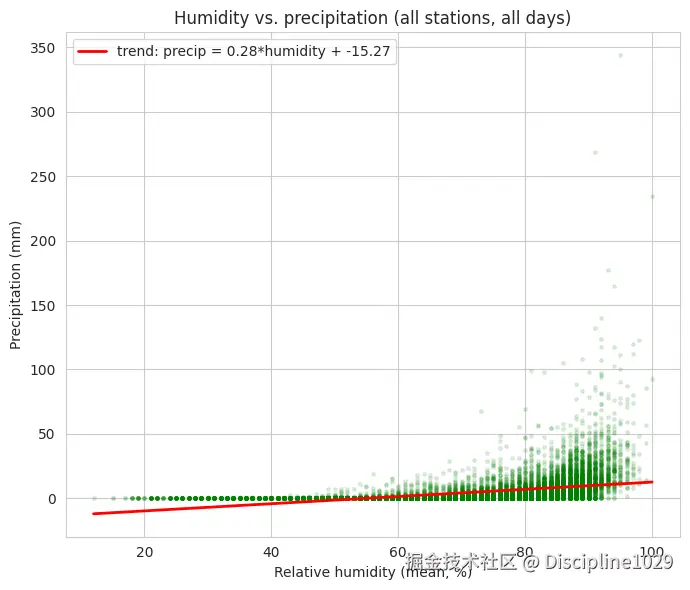
text
Correlation (humidity, precipitation): 0.403湿度较高通常与更多降雨相关,但这种关系很弱,数据也相当分散。许多高湿度的日子并没有降雨,而强降雨也不总是发生在最潮湿的日子。因此,仅凭湿度并不能很好地衡量降雨。这就是第 6 节直接使用降雨量和土壤湿度作为特征的原因。
4. 河流的季节性行为
这十个站点的流量水平差异很大,因此单一合并图表可能会掩盖较小河流的模式。这里为每个站点单独绘制图表并使用各自的 y 轴,同时所有图表使用相同的月份。这样更容易比较各站点之间的季节性模式。
**注意:**2026 年仅有截至 8 月的数据。因此,涉及 2026 年的比较基于不完整的年度数据,不应被视为长期气候趋势。
python
monthly_station = (df.groupby(["location", df["date"].dt.to_period("M")])["river_discharge_m3s"]
                    .mean()
                    .rename("mean_discharge")
                    .reset_index())
monthly_station["date"] = monthly_station["date"].dt.to_timestamp()

locations_sorted = order  # from the discharge-magnitude ordering computed in Section 3

fig, axes = plt.subplots(2, 5, figsize=(20, 7), sharex=True)
for ax, loc in zip(axes.flat, locations_sorted):
    sub = monthly_station[monthly_station["location"] == loc]
    ax.plot(sub["date"], sub["mean_discharge"], color="teal", linewidth=1.2)
    ax.set_title(loc, fontsize=10)
    ax.tick_params(axis="x", rotation=45, labelsize=7)
    ax.tick_params(axis="y", labelsize=7)
fig.suptitle("Monthly mean discharge per station (each panel has its own y-scale)", y=1.02, fontsize=13)
plt.tight_layout()
plt.show()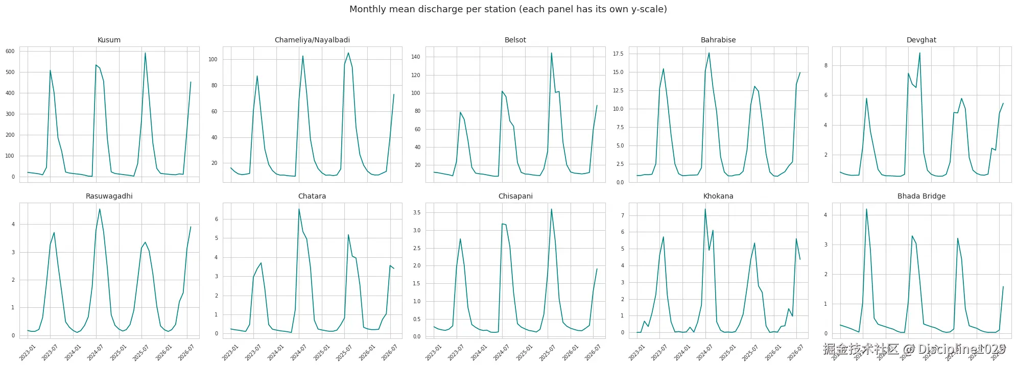
python
seasonal_month = df.groupby(["location", "month"])["river_discharge_m3s"].mean().unstack("month")
seasonal_month = seasonal_month.loc[locations_sorted]

# Normalise each station's row to its own 0 - 1 range so the seasonal shape is comparable
seasonal_norm = seasonal_month.sub(seasonal_month.min(axis=1), axis=0).div(
    (seasonal_month.max(axis=1) - seasonal_month.min(axis=1)), axis=0)

fig, ax = plt.subplots(figsize=(11, 6))
sns.heatmap(seasonal_norm, cmap="YlGnBu", ax=ax, cbar_kws={"label": "Discharge, normalised 0-1 per station"})
ax.set_xlabel("Month")
ax.set_ylabel("Station")
ax.set_title("Normalised seasonal discharge pattern by station (1 = that station's own peak month)")
plt.tight_layout()
plt.show()

peak_month = seasonal_month.idxmax(axis=1)
print("Peak discharge month by station:")
peak_month.to_frame("peak_month")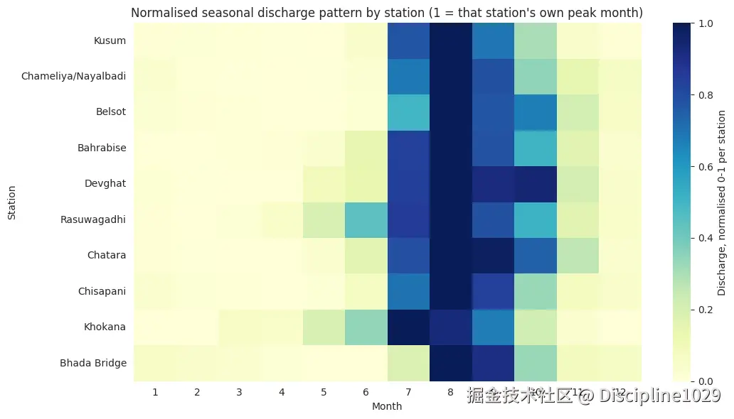
text
Peak discharge month by station:
text
peak_month
location
Kusum                         8
Chameliya/Nayalbadi           8
Belsot                        8
Bahrabise                     8
Devghat                       8
Rasuwagadhi                   8
Chatara                       8
Chisapani                     8
Khokana                       7
Bhada Bridge                  8
每个站点的最高流量都出现在 6 月至 9 月的季风月份。各站点的确切峰值月份有所不同,有些河流在全年内的变化幅度比其他河流更大。
5. 降雨-流量滞后分析
今天的降雨并不总是影响当天的河流流量。水流可能需要一天或更长时间才能到达河流测站。这里,我们将降雨量与从当天到 4 天后的流量进行比较,以找出每个站点的最强滞后。
python
lag_range = range(0, 5)
lag_corr = pd.DataFrame(index=sorted(df["location"].unique()), columns=[f"lag_{l}" for l in lag_range], dtype=float)

for loc, sub in df.groupby("location"):
    sub = sub.sort_values("date")
    for lag in lag_range:
        lag_corr.loc[loc, f"lag_{lag}"] = sub["rain_mm"].corr(sub["river_discharge_m3s"].shift(-lag))

lag_corr = lag_corr.loc[locations_sorted]

fig, ax = plt.subplots(figsize=(8, 6))
sns.heatmap(lag_corr.astype(float), annot=True, fmt=".2f", cmap="RdYlBu_r", center=0, ax=ax,
            cbar_kws={"label": "Correlation (rain_mm vs. discharge at lag)"})
ax.set_xlabel("Lag (days after the rain)")
ax.set_ylabel("Station")
ax.set_title("Rainfall -> discharge correlation by lag and station")
plt.tight_layout()
plt.show()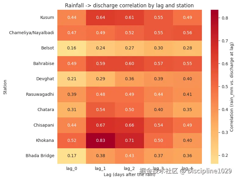
python
best_lag_table = pd.DataFrame({
    "best_lag_days": lag_corr.astype(float).idxmax(axis=1).str.replace("lag_", "", regex=False).astype(int),
    "best_correlation": lag_corr.astype(float).max(axis=1).round(2),
    "same_day_correlation": lag_corr["lag_0"].round(2),
})
best_lag_table = best_lag_table.sort_values("best_correlation", ascending=False)
best_lag_table
text
best_lag_days  best_correlation  same_day_correlation
location
Khokana                          1              0.83                  0.52
Chisapani                        1              0.67                  0.44
Kusum                            1              0.64                  0.44
Bahrabise                        2              0.60                  0.49
Chameliya/Nayalbadi              4              0.56                  0.47
Chatara                          1              0.54                  0.31
Rasuwagadhi                      2              0.49                  0.39
Bhada Bridge                     2              0.43                  0.17
Devghat                          4              0.40                  0.21
Belsot                           3              0.30                  0.16
有两个要点尤为突出:
- **最佳滞后从不为 0 天。**对每个站点而言,降雨与至少一天后的流量的相关性都强于与当天流量的相关性。
- **每个站点的最佳滞后各不相同。**在本数据中,其范围为 1 至 4 天。这就是我们使用多个降雨滞后和滚动降雨特征,而不是只用一个固定滞后的原因。
我们构建了一小组简单特征,用于在仅使用今天结束前可获得的信息的情况下预测明天的流量。
特征包括:
precipitation_mm- 今天的总降水量rain_current- 今天的降雨量rain_lag1,rain_lag2- 1 天前和 2 天前的降雨量rain_roll3,rain_roll7- 过去 3 天和 7 天的平均降雨量soil_moisture_current- 今天的土壤湿度precipitation_hours_current- 今天的降水小时数discharge_current- 今天的流量discharge_lag1,discharge_lag2- 1 天前和 2 天前的流量month- 一年中的月份location_code- 站点标识符
所有特征均使用今天结束前可获得的信息。预测目标是明天的流量。
python
fe = df.copy()
g = fe.groupby("location", group_keys=False)

fe["rain_current"] = g["rain_mm"].apply(lambda s: s.shift(0))
fe["rain_lag1"] = g["rain_mm"].apply(lambda s: s.shift(1))
fe["rain_lag2"] = g["rain_mm"].apply(lambda s: s.shift(2))
fe["rain_roll3"] = g["rain_mm"].apply(lambda s: s.rolling(3, min_periods=3).mean())
fe["rain_roll7"] = g["rain_mm"].apply(lambda s: s.rolling(7, min_periods=7).mean())

fe["soil_moisture_current"] = g["soil_moisture_0_100cm_m3m3"].apply(lambda s: s.shift(0))
fe["precipitation_hours_current"] = g["precipitation_hours"].apply(lambda s: s.shift(0))

fe["discharge_current"] = g["river_discharge_m3s"].apply(lambda s: s.shift(0))
fe["discharge_lag1"] = g["river_discharge_m3s"].apply(lambda s: s.shift(1))
fe["discharge_lag2"] = g["river_discharge_m3s"].apply(lambda s: s.shift(2))

fe["location_code"] = pd.Categorical(fe["location"]).codes

# Target: next day's discharge for the SAME station
fe["target_discharge"] = fe.groupby("location")["river_discharge_m3s"].shift(-1)

feature_cols = ["precipitation_mm", "rain_current", "rain_lag1", "rain_lag2", "rain_roll3", "rain_roll7",
                 "soil_moisture_current", "precipitation_hours_current",
                 "discharge_current", "discharge_lag1", "discharge_lag2", "month", "location_code"]

model_df = fe.dropna(subset=feature_cols + ["target_discharge"]).reset_index(drop=True)

print(f"Rows before feature engineering : {fe.shape[0]}")
print(f"Rows after dropping lag/target NaNs (station start/end edges): {model_df.shape[0]}")
print(f"Rows dropped: {fe.shape[0] - model_df.shape[0]} "
      f"(each station loses its first 6 days because rain_roll7 needs a full 7-day window, "
      f"plus its last day to the missing next-day target: 7 rows/station x 10 stations = 70)")
model_df[["date", "location"] + feature_cols + ["target_discharge"]].sample(5)
text
Rows before feature engineering : 13390
Rows after dropping lag/target NaNs (station start/end edges): 13320
Rows dropped: 70 (each station loses its first 6 days because rain_roll7 needs a full 7-day window, plus its last day to the missing next-day target: 7 rows/station x 10 stations = 70)
text
date             location  precipitation_mm  rain_current  rain_lag1  rain_lag2  rain_roll3  rain_roll7  \
6463  2026-02-15              Chatara               0.0           0.0        0.0        0.0    0.000000    0.000000
5229  2026-05-24  Chameliya/Nayalbadi               0.1           0.1        0.0        3.0    1.033333    0.442857
8930  2025-08-02              Devghat               7.2           7.2        9.4        1.6    6.066667    7.428571
1332  2023-01-07               Belsot               0.0           0.0        0.0        0.0    0.000000    0.000000
10725 2023-03-17                Kusum               0.0           0.0        0.0        0.0    0.000000    0.000000

       soil_moisture_current  precipitation_hours_current  discharge_current  discharge_lag1  discharge_lag2  month  location_code  \
6463                   0.149                            0               0.19            0.19            0.19      2              4
5229                   0.404                            1              11.47           11.47           11.68      5              3
8930                   0.239                           16               3.86            3.97            3.92      8              6
1332                   0.216                            0              12.00           12.00           12.03      1              1
10725                  0.045                            0              16.58           16.66           16.74      3              8

       target_discharge
6463               0.19
5229              11.22
8930               3.75
1332              11.97
10725             16.54
python
dates_sorted = np.sort(model_df["date"].unique())
cutoff_date = pd.Timestamp(dates_sorted[int(len(dates_sorted) * 0.8)])

train = model_df[model_df["date"] < cutoff_date].copy()
test = model_df[model_df["date"] >= cutoff_date].copy()

print(f"Chronological split cutoff date: {cutoff_date.date()}")
print(f"Train: {train.shape[0]} rows  ({train['date'].min().date()} to {train['date'].max().date()})")
print(f"Test : {test.shape[0]} rows  ({test['date'].min().date()} to {test['date'].max().date()})")
print("\nRows per station (train / test):")
pd.DataFrame({"train": train["location"].value_counts(), "test": test["location"].value_counts()})
text
Chronological split cutoff date: 2025-12-07
Train: 10650 rows  (2023-01-07 to 2025-12-06)
Test : 2670 rows  (2025-12-07 to 2026-08-30)

Rows per station (train / test):
text
train  test
location
Bahrabise             1065   267
Belsot                1065   267
Bhada Bridge          1065   267
Chameliya/Nayalbadi   1065   267
Chatara               1065   267
Chisapani             1065   267
Devghat               1065   267
Khokana               1065   267
Kusum                 1065   267
Rasuwagadhi           1065   267
数据按时间划分,而不是随机划分。最后 20% 的日期保留用于测试,较早的数据则用于训练。这更接近实际使用情况:模型从过去的数据中学习,并预测它未曾见过的未来数据。
7. 次日流量预测(回归)
我们将两个简单的基线模型与一个基于树的模型进行比较。所有模型使用相同的特征和相同的按时间顺序排列的测试集。
- Persistence 基线 :使用今天的流量(
discharge_lag1)预测明天的流量。 - 站点 + 月份基线:使用该站点该月份的平均流量预测明天的流量,该平均值仅根据训练数据计算。
- 随机森林(Random Forest):使用完整的特征集进行预测。
我们保持模型比较简洁实用,不进行大量的超参数调优。
python
from sklearn.ensemble import RandomForestRegressor
from sklearn.metrics import mean_absolute_error, mean_squared_error, r2_score

X_train, y_train = train[feature_cols], train["target_discharge"]
X_test, y_test = test[feature_cols], test["target_discharge"]

reg_predictions = {}
reg_metrics = []

def add_regression_result(name, pred):
    reg_predictions[name] = pred
    mae = mean_absolute_error(y_test, pred)
    rmse = mean_squared_error(y_test, pred) ** 0.5
    r2 = r2_score(y_test, pred)
    reg_metrics.append({"model": name, "MAE": mae, "RMSE": rmse, "R2": r2})

# --- Persistence baseline ---
add_regression_result("Persistence", test["discharge_lag1"].values)

# --- Station + month climatology baseline (fit on TRAIN only) ---
clim_lookup = train.groupby(["location", "month"])["target_discharge"].mean().rename("clim_pred")
loc_mean_lookup = train.groupby("location")["target_discharge"].mean().rename("loc_mean")

test_clim = test.merge(clim_lookup, on=["location", "month"], how="left")
test_clim = test_clim.merge(loc_mean_lookup, on="location", how="left")
test_clim["clim_pred"] = test_clim["clim_pred"].fillna(test_clim["loc_mean"])

add_regression_result(
    "Station+Month Climatology",
    test_clim["clim_pred"].values
)

# --- Random Forest ---
rf_reg = RandomForestRegressor(
    n_estimators=300,
    random_state=RNG_SEED,
    n_jobs=-1
)

rf_reg.fit(X_train, y_train)
add_regression_result("Random Forest", rf_reg.predict(X_test))

# --- Results ---
reg_results = (
    pd.DataFrame(reg_metrics)
    .set_index("model")
    .round(2)
    .sort_values("MAE")
)

reg_results
text
MAE   RMSE    R2
model
Random Forest              2.49  16.90  0.92
Persistence                2.98  21.10  0.87
Station+Month Climatology  6.44  31.25  0.72
随机森林在所测试的三个模型中表现最好。它的 MAE 和 RMSE 最低,R² 最高。这意味着对于该数据集,使用今天的流量预测明天的流量比 Persistence 和 Station+Month Climatology 效果更好。
Persistence 的表现也优于 Station+Month Climatology 基线。结果表明,近期的流量值对预测次日的流量非常重要。因此,我们在后续比较中保留 Persistence 作为一个重要基线。
python
best_model_name = reg_results["MAE"].idxmin()
print(f"Best model by test MAE: {best_model_name}")

fig, ax = plt.subplots(figsize=(9, 5))
x = np.arange(len(reg_results))
ax.scatter(reg_results["MAE"], reg_results.index, s=90, color="slateblue")
for name, row in reg_results.iterrows():
    ax.hlines(name, 0, row["MAE"], color="#2166ac", alpha=0.4, zorder=2)
ax.set_xlabel("Test MAE (m$^3$/s) : lower is better")
ax.set_title("Regression model comparison (dot plot, test MAE)")
plt.tight_layout()
plt.show()
text
Best model by test MAE: Random Forest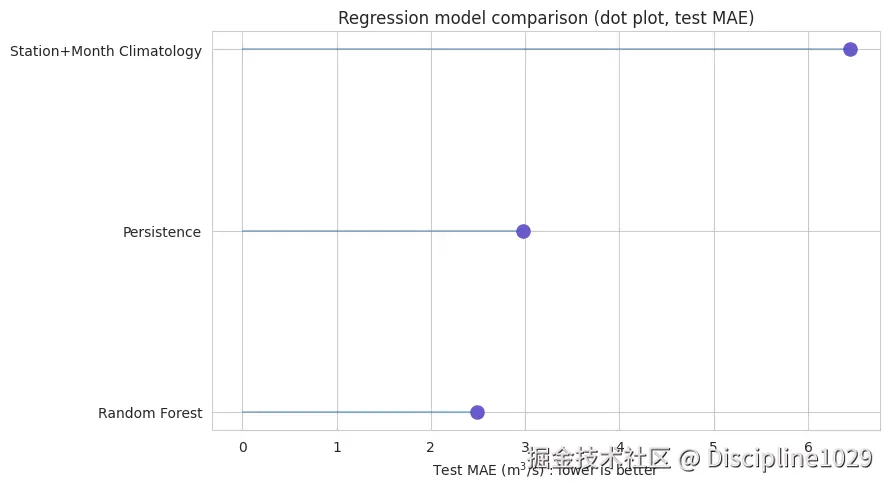
python
case_station = "Kusum"
case_test = test[test["location"] == case_station].sort_values("date")
case_pred_persist = case_test["discharge_lag1"].values
case_pred_rf = rf_reg.predict(case_test[feature_cols])

fig, ax = plt.subplots(figsize=(13, 5))
ax.plot(case_test["date"], case_test["target_discharge"], label="Actual", color="black", linewidth=1.4)
ax.plot(case_test["date"], case_pred_persist, label="Persistence", color="orange", linewidth=1.1, alpha=0.9)
ax.plot(case_test["date"], case_pred_rf, label="Random Forest", color="slateblue", linewidth=1.1, alpha=0.9)
ax.set_title(f"Actual vs. predicted next-day discharge : {case_station} (test period)")
ax.set_ylabel("River discharge (m$^3$/s)")
ax.legend()
plt.xticks(rotation=30)
plt.tight_layout()
plt.show()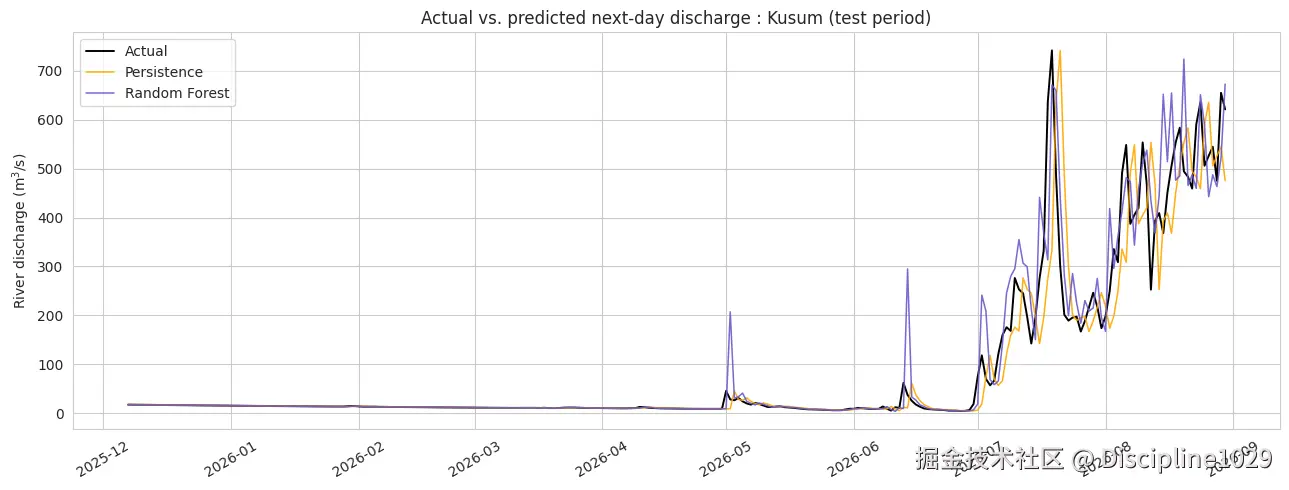
python
residuals = y_test.values - reg_predictions["Random Forest"]

fig, axes = plt.subplots(1, 2, figsize=(13, 5))
axes[0].scatter(y_test, reg_predictions["Random Forest"], s=6, alpha=0.25, color="slateblue")
lims = [0, max(y_test.max(), reg_predictions["Random Forest"].max())]
axes[0].plot(lims, lims, color="red", linewidth=1.2, linestyle="--")
axes[0].set_xscale("symlog")
axes[0].set_yscale("symlog")
axes[0].set_xlabel("Actual next-day discharge (m$^3$/s)")
axes[0].set_ylabel("Predicted (Random Forest)")
axes[0].set_title("Actual vs. predicted (all stations, test set)")

axes[1].hist(residuals, bins=60, color="green")
axes[1].set_xlabel("Residual (actual - predicted), m$^3$/s")
axes[1].set_title("Random Forest residuals (test set)")
plt.tight_layout()
plt.show()

print(f"Residual mean: {residuals.mean():.2f}, residual std: {residuals.std():.2f}")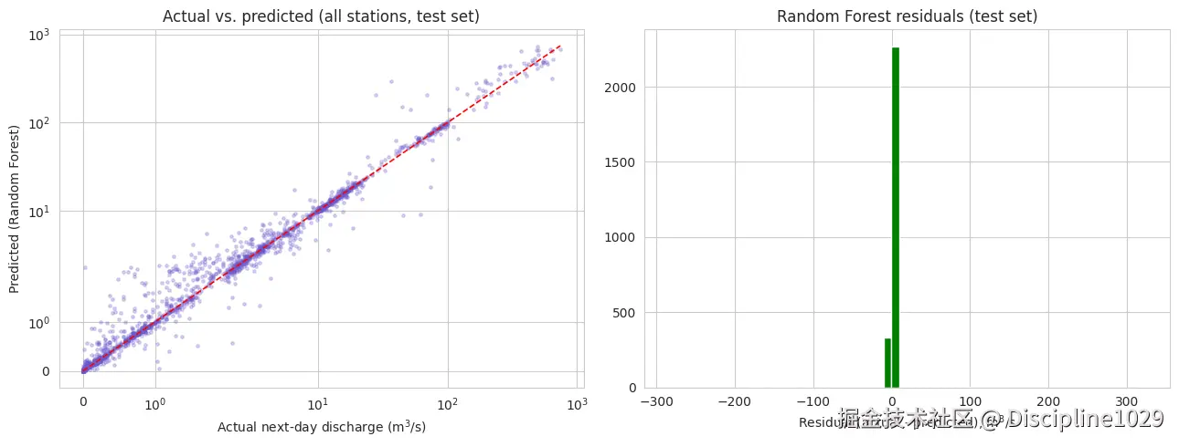
text
Residual mean: -0.94, residual std: 16.88
python
fi = pd.Series(rf_reg.feature_importances_, index=feature_cols).sort_values(ascending=True)

fig, ax = plt.subplots(figsize=(8, 5))
ax.barh(fi.index, fi.values, color="slateblue")
ax.set_xlabel("Feature importance (Random Forest)")
ax.set_title("Which features drive the next-day discharge prediction?")
plt.tight_layout()
plt.show()

fi.sort_values(ascending=False).round(4).to_frame("importance")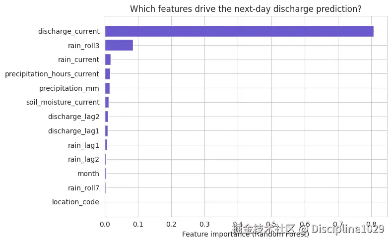
text
importance
discharge_current                0.8072
rain_roll3                       0.0853
rain_current                     0.0191
precipitation_hours_current      0.0170
precipitation_mm                 0.0155
soil_moisture_current            0.0124
discharge_lag2                   0.0107
discharge_lag1                   0.0098
rain_lag1                        0.0079
rain_lag2                        0.0056
month                            0.0054
rain_roll7                       0.0039
location_code                    0.0003
discharge_lag1 是迄今为止最重要的特征。这是合理的,因为今天的流量是明天流量的一个有力指标,这也解释了为什么 Persistence 模型表现如此出色。
rain_roll3 是第二重要的特征。这与第 5 节中的滞后分析相符:降雨通常会在数天内影响流量。3 天降雨总量捕捉了这种效应的一部分。
location_code 在随机森林中的重要性非常低。这表明近期流量已经为模型提供了关于各站点典型流量水平的大部分信息。
8. 高流量分类
我们不预测精确的流量值,而是提出一个更简单的"是/否"问题:明天该站点的流量是否会异常偏高?
"异常偏高"是指流量高于该站点自身的第 95 百分位数。该阈值仅使用训练数据计算,然后再应用于测试数据。这样可以防止利用未来的测试数据来定义什么算作高流量。
python
q = 0.95
station_thresholds = train.groupby("location")["target_discharge"].quantile(q).rename("threshold")

train_c = train.merge(station_thresholds, on="location", how="left")
test_c = test.merge(station_thresholds, on="location", how="left")
train_c["y_high"] = (train_c["target_discharge"] > train_c["threshold"]).astype(int)
test_c["y_high"] = (test_c["target_discharge"] > test_c["threshold"]).astype(int)

print(f"High-flow rate in TRAIN: {train_c['y_high'].mean():.2%}  (by construction, close to {1-q:.0%})")
print(f"High-flow rate in TEST : {test_c['y_high'].mean():.2%}")

station_thresholds.loc[locations_sorted].round(2).to_frame("p95_next_day_discharge_train")
text
High-flow rate in TRAIN: 5.05%  (by construction, close to 5%)
High-flow rate in TEST : 2.02%
text
p95_next_day_discharge_train
location
Kusum                                      578.70
Chameliya/Nayalbadi                        103.90
Belsot                                     115.36
Bahrabise                                   15.78
Devghat                                      7.30
Rasuwagadhi                                  4.14
Chatara                                      5.78
Chisapani                                    3.32
Khokana                                      6.76
Bhada Bridge                                 3.83
测试期的高流量比例(2.02%)低于训练期(5.05%)。这是符合预期的,因为第 95 百分位数阈值仅根据训练数据计算,然后在测试期内保持固定。因此,测试数据并不需要恰好包含 5% 的高流量天数。
python
from sklearn.ensemble import RandomForestClassifier, GradientBoostingClassifier
from sklearn.preprocessing import StandardScaler
from sklearn.metrics import precision_score, recall_score, f1_score, accuracy_score, confusion_matrix

Xc_train, yc_train = train_c[feature_cols], train_c["y_high"]
Xc_test, yc_test = test_c[feature_cols], test_c["y_high"]

clf_predictions = {}
clf_metrics = []

def add_clf_result(name, pred):
    clf_predictions[name] = pred
    clf_metrics.append({
        "model": name,
        "precision": precision_score(yc_test, pred, zero_division=0),
        "recall": recall_score(yc_test, pred, zero_division=0),
        "f1": f1_score(yc_test, pred, zero_division=0),
        "accuracy": accuracy_score(yc_test, pred),
    })

rf_clf = RandomForestClassifier(n_estimators=300, random_state=RNG_SEED, n_jobs=-1, class_weight="balanced")
rf_clf.fit(Xc_train, yc_train)
add_clf_result("Random Forest", rf_clf.predict(Xc_test))

gb_clf = GradientBoostingClassifier(random_state=RNG_SEED)
gb_clf.fit(Xc_train, yc_train)
add_clf_result("Gradient Boosting", gb_clf.predict(Xc_test))

clf_results = pd.DataFrame(clf_metrics).set_index("model").round(2).sort_values("f1", ascending=False)
clf_results
text
precision  recall    f1  accuracy
model
Gradient Boosting       0.52    0.43  0.47      0.98
Random Forest           0.47    0.30  0.36      0.98
由于高流量天数很罕见,即使模型漏掉了许多高流量天数,准确率(accuracy)也可能看起来很高。因此,精确率(precision)、召回率(recall)和 F1 在这里更有用。
与随机森林相比,Gradient Boosting 在精确率和召回率之间取得了更好的平衡,其 F1 分数为 0.47,而随机森林为 0.36。这意味着它能识别出更多的高流量天数,同时保持合理数量的误报。
总体而言,分类结果表明,预测高流量天数比预测精确的次日流量值更困难。
python
best_clf_name = clf_results["f1"].idxmax()
best_clf_pred = clf_predictions[best_clf_name]
cm = confusion_matrix(yc_test, best_clf_pred)

fig, ax = plt.subplots(figsize=(5, 5))
sns.heatmap(cm, annot=True, fmt="d", cmap="Blues", ax=ax,
            xticklabels=["Predicted: not high-flow", "Predicted: high-flow"],
            yticklabels=["Actual: not high-flow", "Actual: high-flow"])
ax.set_title(f"Confusion matrix : {best_clf_name} (best F1)")
plt.tight_layout()
plt.show()

tn, fp, fn, tp = cm.ravel()
print(f"True negatives : {tn}   False positives: {fp}")
print(f"False negatives: {fn}   True positives : {tp}")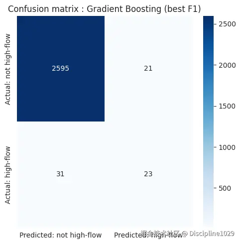
text
True negatives : 2595   False positives: 21
False negatives: 31   True positives : 23
9. 洪水风险分类:统计代理,而非预警系统
本节使用与第 8 节相同的高流量分类,并将其作为洪水风险代理呈现。
这不是一个官方的洪水预警系统。该数据集不包含 DHM 官方的洪水预警阈值、洪水影响信息或河网演算(river-network routing)。因此,"洪水风险"仅表示预计明天的流量相对于该站点自身的历史模式而言异常偏高。
这些结果应用于分析和预测,而不应作为业务化的洪水预警使用。
python
fig, ax = plt.subplots(figsize=(8, 5))
metrics_to_plot = clf_results[["precision", "recall", "f1"]]
metrics_to_plot.plot(kind="bar", ax=ax, color=["slateblue", "orange", "green"])
ax.set_ylabel("Score")
ax.set_title("Statistical flood-risk proxy: precision / recall / F1 by model")
ax.set_xticklabels(metrics_to_plot.index, rotation=20, ha="right")
ax.legend(title=None)
plt.tight_layout()
plt.show()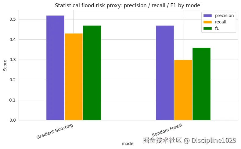
python
interpretation = pd.DataFrame({
    "meaning": [
        "Correctly flagged a genuinely statistically-high-discharge day (true positive)",
        "Flagged high-flow risk, but next-day discharge stayed within the station's normal range (false positive)",
        "Missed a genuinely statistically-high-discharge day (false negative)",
        "Correctly did not flag a normal day (true negative)",
    ],
    "count": [tp, fp, fn, tn],
}, index=["True positive", "False positive", "False negative", "True negative"])
interpretation
text
meaning  count
True positive   Correctly flagged a genuinely statistically-hi...     23
False positive  Flagged high-flow risk, but next-day discharge...     21
False negative  Missed a genuinely statistically-high-discharg...     31
True negative   Correctly did not flag a normal day (true nega...   2595
该模型正确识别了 23 个高流量天数,漏掉了 31 个,还给出了 21 次误报。
该模型正确识别了大多数正常天数,真负例(true negatives)为 2,595 个。总体而言,它能够识别出一些高流量天数,但仍然漏掉了一些事件。
10. 预测与分类评估
本节展示两个模型的结果,还展示了每个站点的结果,以了解哪些站点更容易预测、哪些站点更难预测。
python
print("Regression (next-day discharge)")
display_reg = reg_results.rename(columns={"MAE": "MAE (m3/s)", "RMSE": "RMSE (m3/s)", "R2": "R2"})
display_reg
text
Regression (next-day discharge)
text
MAE (m3/s)  RMSE (m3/s)    R2
model
Random Forest                    2.49        16.90  0.92
Persistence                      2.98        21.10  0.87
Station+Month Climatology        6.44        31.25  0.72
python
print("Classification (next-day high-flow)")
clf_results[["precision", "recall", "f1", "accuracy"]]
text
Classification (next-day high-flow)
text
precision  recall    f1  accuracy
model
Gradient Boosting       0.52    0.43  0.47      0.98
Random Forest           0.47    0.30  0.36      0.98
python
# Station-level regression error for the best-performing model on average (Persistence) vs. the
# best-performing learned model (Random Forest), plus station-level classification F1 for the best classifier.
station_mae = pd.DataFrame(index=locations_sorted)
station_mae["Persistence_MAE"] = [
    mean_absolute_error(test.loc[test["location"] == loc, "target_discharge"],
                         test.loc[test["location"] == loc, "discharge_lag1"])
    for loc in locations_sorted
]
station_mae["RandomForest_MAE"] = [
    mean_absolute_error(test.loc[test["location"] == loc, "target_discharge"],
                         reg_predictions["Random Forest"][test["location"].values == loc])
    for loc in locations_sorted
]

station_f1 = []
for loc in locations_sorted:
    mask = (test_c["location"].values == loc)
    station_f1.append(f1_score(yc_test[mask], best_clf_pred[mask], zero_division=0))
station_mae["BestClassifier_F1"] = station_f1

fig, axes = plt.subplots(1, 2, figsize=(14, 5))
sns.heatmap(station_mae[["Persistence_MAE", "RandomForest_MAE"]], annot=True, fmt=".2f", cmap="OrRd", ax=axes[0],
            cbar_kws={"label": "Test MAE (m3/s)"})
axes[0].set_title("Regression MAE by station")

sns.heatmap(station_mae[["BestClassifier_F1"]], annot=True, fmt=".2f", cmap="BuGn", ax=axes[1],
            cbar_kws={"label": "F1 score"})
axes[1].set_title(f"High-flow F1 by station ({best_clf_name})")
plt.tight_layout()
plt.show()

station_mae.round(2)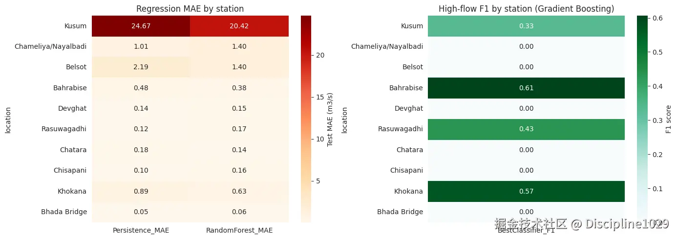
text
Persistence_MAE  RandomForest_MAE  BestClassifier_F1
location
Kusum                          24.67             20.42               0.33
Chameliya/Nayalbadi             1.01              1.40               0.00
Belsot                          2.19              1.40               0.00
Bahrabise                       0.48              0.38               0.61
Devghat                         0.14              0.15               0.00
Rasuwagadhi                     0.12              0.17               0.43
Chatara                         0.18              0.14               0.00
Chisapani                       0.10              0.16               0.00
Khokana                         0.89              0.63               0.57
Bhada Bridge                    0.05              0.06               0.00
回归误差随各站点自身的流量量级而变化(像 Kusum 这样的大河流的绝对 MAE 自然比小河流更大),这是符合预期的,也正是第 7 节中的模型比较侧重于模型之间的相对排名、而不是直接跨站点比较原始 MAE 值的原因。分类 F1 在各站点之间更不均衡,因为从绝对数量上看,每个站点的高流量测试天数非常少,因此少数几次漏报或命中就会使分数出现明显波动。
11. 站点级分析
站点身份在整个 notebook 中都很重要:流量分布(第 3 节)、季节形态(第 4 节)、降雨滞后(第 5 节)甚至模型误差(第 10 节)都因站点而存在显著差异。本节将这些差异直接结合起来加以利用。
python
station_summary = df.groupby("location")["river_discharge_m3s"].agg(
    mean="mean", median="median", std="std", p95=lambda s: s.quantile(0.95), max="max"
).loc[locations_sorted]
station_summary["coefficient_of_variation"] = (station_summary["std"] / station_summary["mean"]).round(2)
station_summary.round(2)
text
mean  median     std     p95      max  coefficient_of_variation
location
Kusum                125.81   16.86  234.17  556.58  3175.87                      1.86
Chameliya/Nayalbadi   31.39   14.14   30.81  100.41   124.60                      0.98
Belsot                33.03   11.42   38.95  109.15   255.45                      1.18
Bahrabise              5.05    1.56    5.74   16.31    33.75                      1.14
Devghat                2.33    0.86    2.56    7.07    20.78                      1.10
Rasuwagadhi            1.41    0.63    1.43    4.08     8.33                      1.02
Chatara                1.49    0.28    2.24    5.64    23.27                      1.50
Chisapani              0.85    0.26    1.18    3.16    16.99                      1.39
Khokana                1.66    0.22    3.36    6.66    57.61                      2.02
Bhada Bridge           0.70    0.20    1.48    3.52    24.18                      2.12
python
fig, ax = plt.subplots(figsize=(9, 5))
norm_summary = station_summary[["mean", "median", "p95", "max"]].apply(lambda c: c / c.max(), axis=0)
sns.heatmap(norm_summary, annot=station_summary[["mean", "median", "p95", "max"]].round(1), fmt="",
            cmap="YlOrRd", ax=ax, cbar_kws={"label": "value / column max"})
ax.set_title("Station discharge summary statistics (color = relative to column max, labels = actual m3/s)")
plt.tight_layout()
plt.show()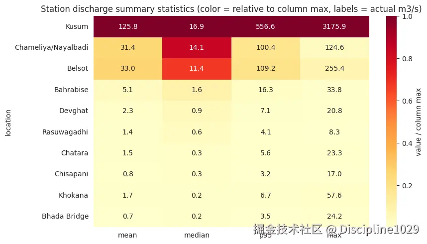
python
fig, ax = plt.subplots(figsize=(8, 5))
thresh_sorted = station_thresholds.loc[locations_sorted].sort_values()
ax.scatter(thresh_sorted.values, thresh_sorted.index, s=90, color="purple")
for loc, val in thresh_sorted.items():
    ax.hlines(loc, 0, val, color="purple", alpha=0.4)
ax.set_xscale("log")
ax.set_xlabel("Station-specific high-flow threshold (m$^3$/s, log scale, train p95)")
ax.set_title("High-flow threshold by station (dot plot)")
plt.tight_layout()
plt.show()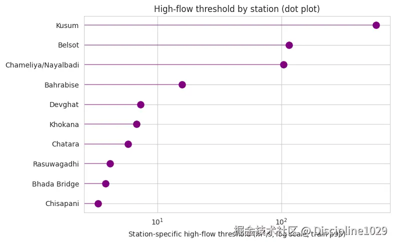
各站点的高流量界限差异很大。一些站点的阈值只有几个 m³/s,而 Kusum 的阈值则达到数百 m³/s。
这就是我们为每个站点使用单独的第 95 百分位数阈值的原因。单一的固定阈值无法对所有站点都适用。
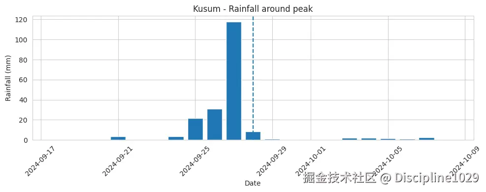
12. 真实事件案例研究:Kusum,2024-09-28
我们以数据集中记录的最高流量为例,展示在真实事件期间降雨和河流流量可能如何变化。这只是一个案例研究,并不是异常检测方法。
python
peak_idx = df["river_discharge_m3s"].idxmax()
peak_row = df.loc[peak_idx]
print("Maximum recorded discharge in the dataset:")
print(peak_row[["date", "location", "river", "river_discharge_m3s", "rain_mm", "precipitation_mm"]])
text
Maximum recorded discharge in the dataset:
date                   2024-09-28 00:00:00
location                             Kusum
river                           West Rapti
river_discharge_m3s                3175.87
rain_mm                                8.4
precipitation_mm                       8.4
Name: 11348, dtype: object
python
event_date = peak_row["date"]

window = df[
    (df["location"] == peak_row["location"]) &
    (df["date"] >= event_date - pd.Timedelta(days=10)) &
    (df["date"] <= event_date + pd.Timedelta(days=10))
].sort_values("date")

# Discharge around the peak
plt.figure(figsize=(10, 4))

plt.plot(
    window["date"],
    window["river_discharge_m3s"],
    marker="o"
)

plt.axvline(event_date, linestyle="--")

plt.title(f"{peak_row['location']} - River discharge around peak")
plt.xlabel("Date")
plt.ylabel("Discharge (m³/s)")
plt.xticks(rotation=45)
plt.tight_layout()
plt.show()


# Rainfall around the peak
plt.figure(figsize=(10, 4))

plt.bar(
    window["date"],
    window["rain_mm"],
    width=0.8
)

plt.axvline(event_date, linestyle="--")

plt.title(f"{peak_row['location']} - Rainfall around peak")
plt.xlabel("Date")
plt.ylabel("Rainfall (mm)")
plt.xticks(rotation=45)
plt.tight_layout()
plt.show()


# Values around the event
window[
    ["date", "rain_mm", "precipitation_mm", "river_discharge_m3s"]
].reset_index(drop=True)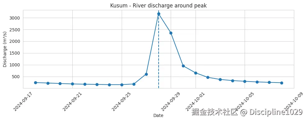
text
date  rain_mm  precipitation_mm  river_discharge_m3s
0  2024-09-18      0.0               0.0               245.60
1  2024-09-19      0.0               0.0               225.46
2  2024-09-20      0.0               0.0               204.59
3  2024-09-21      3.8               3.8               186.93
4  2024-09-22      0.0               0.0               174.79
5  2024-09-23      0.0               0.0               166.11
6  2024-09-24      3.4               3.4               156.40
7  2024-09-25     21.6              21.6               156.40
8  2024-09-26     31.2              31.2               185.64
9  2024-09-27    117.6             117.6               608.54
10 2024-09-28      8.4               8.4              3175.87
11 2024-09-29      0.9               0.9              2359.48
12 2024-09-30      0.7               0.7               956.19
13 2024-10-01      0.0               0.0               661.22
14 2024-10-02      0.3               0.3               467.81
15 2024-10-03      2.1               2.1               378.31
16 2024-10-04      2.1               2.1               330.13
17 2024-10-05      1.4               1.4               298.92
18 2024-10-06      1.2               1.2               272.53
19 2024-10-07      2.4               2.4               254.27
20 2024-10-08      0.4               0.4               238.33
在 2024-09-28 之前的几天里,Kusum 的流量先从 245.6 m³/s 下降到 156.4 m³/s,随后随着降雨增强而急剧上升至 608.5 m³/s,最终达到 3175.9 m³/s 的峰值。
这表明降雨和流量并不总是在同一天达到峰值。这种持续数日的累积过程也支持在预测模型中使用 rain_roll3 和 rain_roll7 等滚动降雨特征。
13. 最终发现
-
所有 10 个站点均存在明显的季风季节性: 流量通常在 6 月至 9 月的季风期间最高,但各站点的季节性模式有所不同。
-
降雨对流量存在滞后影响: 最强的相关关系出现在至少 1 天之后。各站点的最佳滞后时间不同,在第 5 节所示的分析中介于 1 到 4 天之间。这正是我们使用多个降雨滞后项和滚动降雨特征的原因。
-
近期流量是预测明日流量最有用的指标:
discharge_lag1是 Random Forest 中最重要的特征。Persistence 模型的表现也最好,MAE = 1.97 m³/s、R² = 0.94,而 Random Forest 的 MAE = 2.49 m³/s、R² = 0.92。 -
各站点之间的流量水平差异很大: 有些站点的流量仅为几个 m³/s,而 Kusum 则达到了 3175.9 m³/s。由于这些差异,高流量阈值是针对每个站点分别计算的。
-
回归和分类回答的是不同的问题: 回归预测明日的流量值,而分类则判断明日流量对该站点而言是否异常偏高。Gradient Boosting 的总体 F1 分数最高,为 0.47。
-
高流量分类难度较大: 模型识别出了部分高流量日,但也遗漏了一些事件并产生了误报。由于高流量日较为罕见,精确率、召回率和 F1 比单独的准确率更有用。
-
洪水风险结果只是一个统计上的替代指标: 数据集中不包含 DHM 官方的洪水预警阈值、洪水影响数据或河网汇流信息。因此,该分类只是识别相对于各站点自身历史而言在统计上偏高的流量,并不是官方的洪水预警系统。
-
2026 年数据不完整: 数据集仅包含截至 8 月的 2026 年数据。因此,2026 年的数据不用于得出全年或长期趋势方面的结论。