机器学习之线性回归

线性回归

回归问题：预测连续的数值输出，如房价、温度、股票等。

核心思想：线性回归就是用一条直线（多元时是超平面）去拟合数据点，使预测误差最小，从而刻画输入特征与连续目标值之间的线性关系（即：找到数据背后的线性关系）。
数学表达式（ŷ为预测值，x为特征值）：
- 单变量：ŷ = ax + b
- 多变量（多元线性回归）：ŷ = Wᵀ X + b
- 优化目标 ：找到最优参数【a（斜率）和b（截距）】，使模型预测最准确，通常会使用**最小二乘法（通常选此）或 梯度下降（数据量大情况选此）**。
最小二乘法：求得最优参数
- 数学原理（直觉三步）：
  - 算误差：每个点预测值（ŷ）与真实值（y）的差。
  - 平方：将误差平方，避免正负抵消，并放大大误差的影响。
  - 求和最小化：把所有平方误差加总，寻找让这个总和最小的直线。
- 参数求解 ：
  
  对于n个样本，损失函数定义为：
  
  L=1n∑i=1n(yi−y^i)2 L = \frac{1}{n} \sum_{i=1}^{n} (y_i - \hat{y}_i)^2 L=n1i=1∑n(yi−y^i)2
  
  通过对a和b求偏导并令其为0，可以得到解析解：
  
  a=∑(xi−xˉ)(yi−yˉ)∑(xi−xˉ)2 a = \frac{\sum (x_i - \bar{x})(y_i - \bar{y})}{\sum (x_i - \bar{x})^2} a=∑(xi−xˉ)2∑(xi−xˉ)(yi−yˉ)
  
  b=yˉ−axˉ b = \bar{y} - a\bar{x} b=yˉ−axˉ
评估模型：

方法一 ：均方误差（MSE）

MSE=1N∑n=1N(y^n−yn)2 MSE = \frac{1}{N} \sum_{n=1}^{N} (\hat{y}_n - y_n)^2 MSE=N1n=1∑N(y^n−yn)2
- 概念：MSE衡量预测值（ŷ）与真实值（y）之间的平方平均数
- MSE越小，模型预测越准确
- 缺点：对异常值敏感，因为平方会放大较大误差的影响
方法二 ：决定系数（R²）

R2=1−∑i=1n(yi−y^i)2∑i=1n(yi−yˉ)2 R^2 = 1 - \frac{\sum_{i=1}^{n}(y_i - \hat{y}i)^2}{\sum{i=1}^{n}(y_i - \bar{y})^2} R2=1−∑i=1n(yi−yˉ)2∑i=1n(yi−y^i)2
- 概念：目标变量（y）的总波动中，有多大比例能被模型解释；越接近 1，说明模型对数据波动的拟合越好
- 举例：R²=0.8，表示模型解释了80%的数据方差
- 特点：更直观理解模型好坏

案例：糖尿病病情发展预测

采用sklearn内部数据，其含义如下：

age	sex	bmi	bp	s1	s2	s3	s4	s5	s6	target
年龄	性别	身体质量指数	平均血压	总血清胆固醇	低密度脂蛋白胆固醇	高密度脂蛋白胆固醇	总胆固醇与HDL胆固醇的比值	血清甘油三酯水平的对数值	血糖水平	目标变量

单变量线性回归：

python 复制代码

import pandas as pd
from sklearn.datasets import load_diabetes
from sklearn.linear_model import LinearRegression
from sklearn.metrics import mean_squared_error, r2_score
from sklearn.model_selection import train_test_split

# 1.1、准备数据
database = load_diabetes() # 加载数据集
# 构建二维表格（Pandas DataFrame）
df = pd.DataFrame(database.data,columns=database.feature_names)
df['target'] = database.target
# 确认数据
x=df[['bmi']] # 特征：体质指数
y=df['target'] # 目标：一年后糖尿病病情的定量进展指标
# 查看数据
print(df.head(7)) # 查看数据
print(f"列表名称：{df.columns.tolist()}") # 查看列名

# 1.2、划分训练集和测试集
x_train,x_test,y_train,y_test = train_test_split(
    x,y,test_size=0.2,random_state=42
)

# 2、模型
model = LinearRegression()

# 3、使用训练数据拟合模型（找到最优参数）
model.fit(x_train,y_train)

# 4、使用训练好的模型进行预测
predictions = model.predict(x_test)

# 查看模型参数
print(f"斜率：{model.coef_}")
print(f"截距：{model.intercept_}")

# 模型评估
# 方法一：均方误差（MSE）
mse = mean_squared_error(y_test,predictions)
print(f"均方误差（MSE）：{mse:.2f}")
# 方法二：决定系数（R²）
r2 = r2_score(y_test,predictions)
print(f"决定系数（R²）:{r2:.2f}")
if r2 > 0.9:
    print("模型拟合非常好！")
elif r2 > 0.7:
    print("模型拟合良好")
else:
    print("模型需改进")
-----------------------------------------------------------------------
        age       sex       bmi        bp  ...        s4        s5        s6  target
0  0.038076  0.050680  0.061696  0.021872  ... -0.002592  0.019907 -0.017646   151.0
1 -0.001882 -0.044642 -0.051474 -0.026328  ... -0.039493 -0.068332 -0.092204    75.0
2  0.085299  0.050680  0.044451 -0.005670  ... -0.002592  0.002861 -0.025930   141.0
3 -0.089063 -0.044642 -0.011595 -0.036656  ...  0.034309  0.022688 -0.009362   206.0
4  0.005383 -0.044642 -0.036385  0.021872  ... -0.002592 -0.031988 -0.046641   135.0
5 -0.092695 -0.044642 -0.040696 -0.019442  ... -0.076395 -0.041176 -0.096346    97.0
6 -0.045472  0.050680 -0.047163 -0.015999  ... -0.039493 -0.062917 -0.038357   138.0

[7 rows x 11 columns]
列表名称：['age', 'sex', 'bmi', 'bp', 's1', 's2', 's3', 's4', 's5', 's6', 'target']
斜率：[998.57768914]
截距：152.00335421448167
均方误差（MSE）：4061.83
决定系数（R²）:0.23
模型需改进
-----------------------------------------------------------------------

多元线性回归：

python 复制代码

import pandas as pd
from sklearn.datasets import load_diabetes
from sklearn.linear_model import LinearRegression
from sklearn.metrics import mean_squared_error, r2_score
from sklearn.model_selection import train_test_split

# 1.1、准备数据
database = load_diabetes() # 加载数据集
# 构建二维表格（Pandas DataFrame）
df = pd.DataFrame(database.data,columns=database.feature_names)
df['target'] = database.target
# 确认数据
x=df[['age','sex','bmi','bp','s1','s2','s3','s4','s5','s6']]
y=df['target'] # 目标：一年后糖尿病病情的定量进展指标
# 查看信息
print(f"列表名称：{df.columns.tolist()}") # 查看列名

# 1.2、划分训练集和测试集
x_train,x_test,y_train,y_test = train_test_split(
    x,y,test_size=0.2,random_state=71
)

# 数据标准化★★★
from sklearn.preprocessing import StandardScaler
scaler = StandardScaler()
x_train_scaled = scaler.fit_transform(x_train) # fit_transform（计算均值方差并转换）  ★
x_test_scaled = scaler.transform(x_test) # 绝对不能 fit  ★

# 2、模型
model = LinearRegression()

# 3、使用训练数据拟合模型（找到最优参数）
model.fit(x_train_scaled,y_train) # ★

# 4、使用训练好的模型进行预测
predictions = model.predict(x_test_scaled) # ★

# 查看模型参数
print(f"斜率：{model.coef_}")
print(f"截距：{model.intercept_}")

# 6、模型评估
mse = mean_squared_error(y_test, predictions)
r2 = r2_score(y_test, predictions)
print("-" * 30)
print(f"均方误差（MSE）：{mse:.2f}")
print(f"决定系数（R²）:{r2:.2f}")

# 7、模型解释（寻找影响力最大的特征）
max_abs_coef = 0
best_feature = ""
feature_names = ['age','sex','bmi','bp','s1','s2','s3','s4','s5','s6']

for name, coef in zip(feature_names, model.coef_):
    current_abs = abs(coef)
    print(f"{name}的系数：{coef:.2f} (绝对值：{current_abs:.2f})")
    if current_abs > max_abs_coef:
        max_abs_coef = current_abs
        best_feature = name

print("-" * 30)
print(f"影响力最大的特征是：{best_feature}，其绝对值为：{max_abs_coef:.2f}")
---------------------------------------------------------------------
列表名称：['age', 'sex', 'bmi', 'bp', 's1', 's2', 's3', 's4', 's5', 's6', 'target']
斜率：[ -0.1072002  -11.94567104  27.98645676  14.94664879 -35.41653719
  23.07662268   4.82519932   6.2730565   37.01522646   0.25761677]
截距：152.90084985835693
------------------------------
均方误差（MSE）：2967.10
决定系数（R²）:0.45
age的系数：-0.11 (绝对值：0.11)
sex的系数：-11.95 (绝对值：11.95)
bmi的系数：27.99 (绝对值：27.99)
bp的系数：14.95 (绝对值：14.95)
s1的系数：-35.42 (绝对值：35.42)
s2的系数：23.08 (绝对值：23.08)
s3的系数：4.83 (绝对值：4.83)
s4的系数：6.27 (绝对值：6.27)
s5的系数：37.02 (绝对值：37.02)
s6的系数：0.26 (绝对值：0.26)
------------------------------
影响力最大的特征是：s5，其绝对值为：37.02
---------------------------------------------------------------------

fit_transform（拟合/学习+转换） = 学习规则 + 应用规则（用于训练集）

transform（转换） = 仅应用已有的规则（用于测试集和新数据）

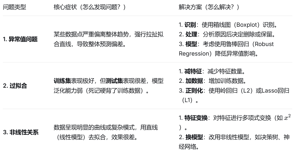
常见问题与解决方案