深度学习实战-基于EfficientNetB0的鞋类品牌图像分类模型

🤵‍♂️ 个人主页：@艾派森的个人主页

✍🏻作者简介：Python学习者

🐋 希望大家多多支持，我们一起进步！😄

如果文章对你有帮助的话，

欢迎评论 💬点赞👍🏻 收藏 📂加关注+

---

目录

1.项目背景

2.数据集介绍

3.技术工具

4.实验过程

4.1导入数据

4.2数据预处理

4.3数据可视化

4.4构建模型

4.5训练模型

4.6模型评估

5.总结

源代码

---

1.项目背景

随着电子商务与时尚零售产业的数字化转型，线上商品图像的自动识别与精准分类已成为打造智能推荐系统、优化视觉搜索以及提升供应链管理效率的核心技术支撑。在鞋类电商领域，同类目商品在外观设计、线条结构及材质纹理上往往具有极高的相似性，加之拍摄视角、光照条件与背景环境的多样变化，使得人工标注与传统图像特征提取方法的效率和准确率难以满足大规模商业应用的需求。为了实现对阿迪达斯、匡威及耐克等主流鞋类品牌的高效自动识别，本项目基于深度学习技术，探索利用卷积神经网络在复杂图像特征提取方面的显著优势。通过引入预训练的 EfficientNetB0 架构，并结合定制化的数据预处理与模型正则化策略，构建了一个具备高泛化能力的鞋类品牌分类模型，旨在为鞋支商品的自动归类、图像检索及智能运维提供可靠的技术解决方案与理论参考。

2.数据集介绍

本实验数据集来源于Kaggle，数据集包含两个文件夹：一个包含测试数据，另一个包含训练数据。测试集与训练集的划分比例为 0.14，测试集包含 114 张图像，训练集包含 711 张图像。
图像分辨率为 240x240 像素，颜色模式为 RGB。两个文件夹均包含 3 个类别：

• 阿迪达斯
• 匡威
• 耐克

3.技术工具

Python版本:3.9

代码编辑器：jupyter notebook

4.实验过程

4.1导入数据

在搭建深度学习模型之前，首先需要导入系统基础库、数据处理工具以及 TensorFlow/Keras 深度学习框架相关组件，为后续的图像处理、数据清洗、模型构建及指标评估提供完整的功能支持。通过配置 Warning 过滤机制，可以确保在代码运行过程中屏蔽无意义的框架提示，保持控制台输出的简洁明了。

# ----------------------------------------------------------------------
# 1. 导入系统基础库与路径处理工具
# ----------------------------------------------------------------------
import os
import time
import shutil
import pathlib
import itertools
from PIL import Image
# ----------------------------------------------------------------------
# 2. 导入数据分析、处理与绘图可视化工具
# ----------------------------------------------------------------------
import cv2
import numpy as np
import pandas as pd
import seaborn as sns
sns.set_style('darkgrid') # 设置绘图主题为暗色网格风格
import matplotlib.pyplot as plt
from sklearn.model_selection import train_test_split
from sklearn.metrics import confusion_matrix, classification_report
# ----------------------------------------------------------------------
# 3. 导入 TensorFlow 深度学习框架及网络层组件
# ----------------------------------------------------------------------
import tensorflow as tf
from tensorflow import keras
from tensorflow.keras.models import Sequential
from tensorflow.keras.optimizers import Adam, Adamax
from tensorflow.keras.metrics import categorical_crossentropy
from tensorflow.keras.preprocessing.image import ImageDataGenerator
from tensorflow.keras.layers import Conv2D, MaxPooling2D, Flatten, Dense, Activation, Dropout, BatchNormalization
from tensorflow.keras import regularizers
# ----------------------------------------------------------------------
# 4. 忽略不必要的警告信息，保持输出界面整洁
# ----------------------------------------------------------------------
import warnings
warnings.filterwarnings("ignore")

依赖库导入完毕后，接下来对训练集与测试集目录下的图像文件进行扫描与读取。通过遍历不同品牌分类文件夹，动态提取每张鞋类图像的完整文件路径及其对应的品牌类别标签，并将这些信息映射拼接为 Pandas Dataframe 结构，从而将无序的磁盘文件组织成结构化的数据框，方便后续对数据流进行统一管理与批量加载。

# ----------------------------------------------------------------------
# 5. 读取并构建训练集路径与标签 Dataframe
# ----------------------------------------------------------------------
train_dir = '/kaggle/input/nike-adidas-and-converse-imaged/train'
filepaths = []
labels = []
# 遍历训练集子目录提取图像路径与对应的类别标签
folds = os.listdir(train_dir)
for fold in folds:
    foldpath = os.path.join(train_dir, fold)
    filelist = os.listdir(foldpath)
    for file in filelist:
        fpath = os.path.join(foldpath, file)
        filepaths.append(fpath)
        labels.append(fold)

# 将图像路径与类别标签合并为一维 Series 并拼接为训练数据框
Fseries = pd.Series(filepaths, name= 'filepaths')
Lseries = pd.Series(labels, name='labels')
train_df = pd.concat([Fseries, Lseries], axis= 1)
# ----------------------------------------------------------------------
# 6. 读取并构建测试集路径与标签 Dataframe
# ----------------------------------------------------------------------
test_dir = '/kaggle/input/nike-adidas-and-converse-imaged/test'
filepaths = []
labels = []
# 遍历测试集子目录提取图像路径与对应的类别标签
folds = os.listdir(test_dir)
for fold in folds:
    foldpath = os.path.join(test_dir, fold)
    filelist = os.listdir(foldpath)
    for file in filelist:
        fpath = os.path.join(foldpath, file)
        filepaths.append(fpath)
        labels.append(fold)

# 将图像路径与类别标签合并为一维 Series 并拼接为测试数据框
Fseries = pd.Series(filepaths, name= 'filepaths')
Lseries = pd.Series(labels, name='labels')
test_df = pd.concat([Fseries, Lseries], axis= 1)
# 输出查看构建完成的测试集数据框结构
test_df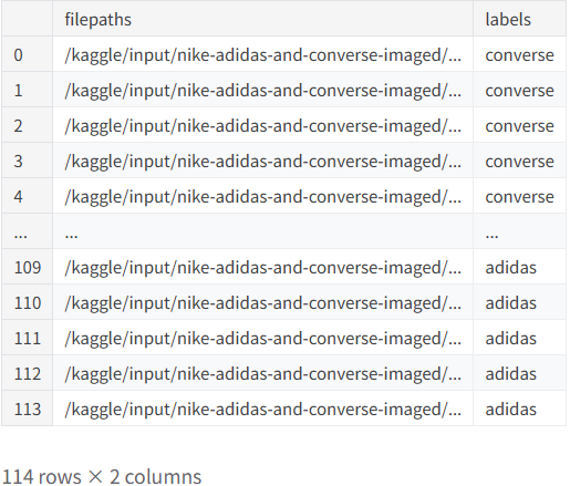

4.2数据预处理

构建好包含图像路径与标签的表格数据后，需要对其进行划分与标准化生成处理。首先利用 train_test_split 将原始测试集数据进一步按 60:40 的比例随机划分为验证集与测试集，确保模型在训练过程中有独立的验证数据进行超参数调优，同时保留不参与训练的最终测试数据。紧接着设定统一的批次大小（batch_size = 16）与图像输入尺寸（224×224×3），并通过 TensorFlow 的 ImageDataGenerator 配合 flow_from_dataframe 建立高效的数据批次生成流，实现图像数据的按需动态加载与多分类独热编码（Categorical）转换。

# ----------------------------------------------------------------------
# 1. 切分验证集与测试集数据框
# ----------------------------------------------------------------------
# 将原始 test_df 按 6:4 的比例划分为验证集 (valid_df) 与最终测试集 (test_df)
valid_df, test_df = train_test_split(test_df, train_size= 0.6, shuffle= True, random_state= 123)
# ----------------------------------------------------------------------
# 2. 设定图像尺寸与训练批次参数
# ----------------------------------------------------------------------
batch_size = 16 # 批次大小
img_size = (224, 224) # 图像输入目标分辨率
channels = 3 # 图像色彩通道数（RGB）
img_shape = (img_size[0], img_size[1], channels)
# ----------------------------------------------------------------------
# 3. 实例化 ImageDataGenerator 数据生成器并构建数据流
# ----------------------------------------------------------------------
tr_gen = ImageDataGenerator()
ts_gen = ImageDataGenerator()
# 构建训练集批次生成器（保持打乱状态以增强训练随机性）
train_gen = tr_gen.flow_from_dataframe( train_df, x_col= 'filepaths', y_col= 'labels', target_size= img_size, class_mode= 'categorical',
                                    color_mode= 'rgb', shuffle= True, batch_size= batch_size)
# 构建验证集批次生成器
valid_gen = ts_gen.flow_from_dataframe( valid_df, x_col= 'filepaths', y_col= 'labels', target_size= img_size, class_mode= 'categorical',
                                    color_mode= 'rgb', shuffle= True, batch_size= batch_size)
# 构建测试集批次生成器（关闭打乱操作，确保预测结果与真实标签一一对应）
test_gen = ts_gen.flow_from_dataframe( test_df, x_col= 'filepaths', y_col= 'labels', target_size= img_size, class_mode= 'categorical',
                                    color_mode= 'rgb', shuffle= False, batch_size= batch_size)

4.3数据可视化

为了验证图像数据流加载的正确性以及直观了解数据集中的样本特征，有必要在模型训练前对批次图像及其标注进行可视化展示。代码通过获取数据生成器中的类别映射字典得到具体的品牌名称列表，并从训练流中提取一个 Batch（包含 16 张图像）的数据。随后，对图像像素值进行归一化处理（缩放到 0 至 1 范围）以适配绘图要求，并结合独热编码还原出对应的品牌标签，利用 4×4 的网格布局进行批量绘制展示。

# ----------------------------------------------------------------------
# 动态提取批次数据并进行图像可视化
# ----------------------------------------------------------------------
g_dict = train_gen.class_indices      # 获取类别与索引的映射字典 {'class': index}
classes = list(g_dict.keys())       # 提取所有类别名称列表
images, labels = next(train_gen)      # 从训练批次生成器中获取一个 Batch 的图像与标签数据
plt.figure(figsize= (20, 20))
# 循环绘制网格中的 16 张样本图像
for i in range(16):
    plt.subplot(4, 4, i + 1)
    image = images[i] / 255       # 将像素值归一化至 [0, 1] 范围以便清晰显示
    plt.imshow(image)
    index = np.argmax(labels[i])  # 提取独热编码中最大值的索引
    class_name = classes[index]   # 根据索引获取具体的品牌类别名称
    plt.title(class_name, color= 'blue', fontsize= 12)
    plt.axis('off')               # 隐藏坐标轴线
plt.show()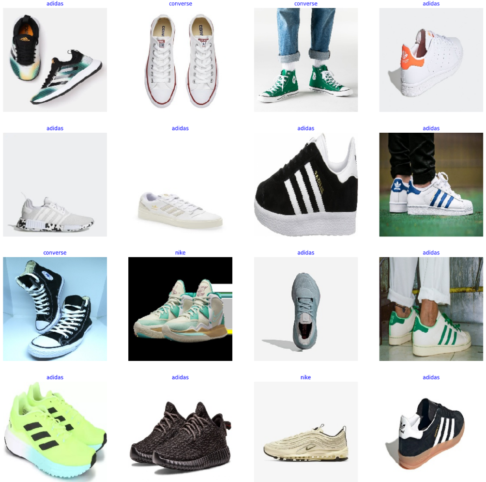

4.4构建模型

在模型构建阶段，代码采用了迁移学习架构，选取 EfficientNetB0 作为主干特征提取网络，并借助在 ImageNet 上预训练的权重来捕获图像的底层通用特征。为了适配鞋类品牌的多分类任务，网络在 EfficientNetB0 主干的基础上采用 Sequential 顺序结构，依次叠加了 BatchNormalization 批量归一化层、带有 L1/L2 正则化约束的 Dense 隐藏层、Dropout 随机失活层以及最后基于 Softmax 的输出分类层。模型编译阶段选用 Adamax 优化器，损失函数采用适合多分类任务的 categorical_crossentropy，并通过 model.summary() 打印输出整个网络的结构细节与参数量分布。

# ----------------------------------------------------------------------
# 1. 设置输入维度与类别数量
# ----------------------------------------------------------------------
img_size = (224, 224)
channels = 3
img_shape = (img_size[0], img_size[1], channels)
class_count = len(list(train_gen.class_indices.keys())) # 根据数据生成器自动获取分类类别数
# ----------------------------------------------------------------------
# 2. 加载 EfficientNetB0 预训练主干网络
# ----------------------------------------------------------------------
# 移除顶层分类器，使用全局最大池化 (pooling='max') 提取特征图特征
base_model = tf.keras.applications.efficientnet.EfficientNetB0(include_top= False, weights= "imagenet", input_shape= img_shape, pooling= 'max')
# base_model.trainable = False
# ---------------------------------------------------------------------
# 3. 组装顶层分类网络结构
# ----------------------------------------------------------------------
model = Sequential([
    base_model,
    BatchNormalization(axis= -1, momentum= 0.99, epsilon= 0.001), # 批标准化加速网络收敛
    Dense(256, kernel_regularizer= regularizers.l2(l= 0.016), activity_regularizer= regularizers.l1(0.006),
                bias_regularizer= regularizers.l1(0.006), activation= 'relu'), # 结合 L1/L2 正则化的全连接层
    Dropout(rate= 0.45, seed= 123), # 高丢弃率 Dropout 抑制作业过拟合
    Dense(class_count, activation= 'softmax') # 多分类输出层
])
# ---------------------------------------------------------------------
# 4. 编译模型并查看网络结构
# ----------------------------------------------------------------------
model.compile(Adamax(learning_rate= 0.001), loss= 'categorical_crossentropy', metrics= ['accuracy'])
# 打印模型架构摘要
model.summary()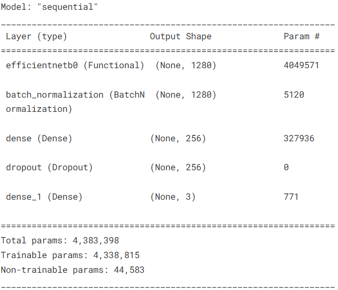

通过引入预训练主干网络并结合多重正则化手段，该架构在保证深层特征提取能力的同时，极大降低了在小样本数据上发生过拟合的风险。精心设计的梯度更新约束与优化器配置，为后续的高效迭代与平稳收敛提供了坚实保障。

4.5训练模型

在确定好模型架构与优化策略后，进入模型的迭代训练阶段。代码重新指定了训练时每个批次的样本数量（batch_size = 20）以及总迭代轮数（epochs = 20）。通过调用 fit 函数传入构建好的训练集与验证集生成器，模型将在指定的轮数内逐步更新权重参数，实时监控训练集与验证集上的损失值与准确率变化，以实现参数的稳健收敛。

# ----------------------------------------------------------------------
# 配置训练参数并启动模型迭代训练
# ----------------------------------------------------------------------
batch_size = 20   # 设置训练过程中的批次大小
epochs =  20      # 设置总迭代轮数
# 启动训练流，依次传入训练生成器与验证生成器进行 20 轮迭代
history = model.fit(x= train_gen, epochs= epochs, verbose= 1, validation_data= valid_gen, 
                    validation_steps= None, shuffle= False)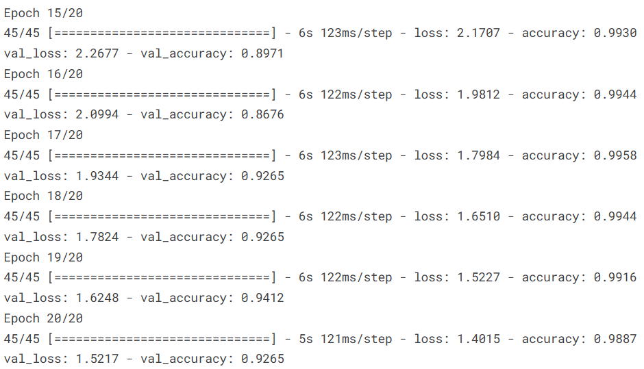

4.6模型评估

模型训练完成后，需要从多个维度对模型的泛化能力与分类性能进行系统化评估。本节评估分为四个核心环节：首先绘制训练与验证阶段的损失值及准确率曲线，精确定位最优迭代轮次；其次动态计算适配测试集的数据批次，并针对训练集、验证集和测试集分别评估整体损失与准确率；随后基于预测结果绘制混淆矩阵，直观展示各类鞋类品牌间的误判分布情况；最后生成详细的分类报告，给出精准率（Precision）、召回率（Recall）及 F1 分数（F1-Score）等量化指标。

1. 训练与验证曲线可视化

通过提取训练日志中的损失与准确率数据，结合散点标记精准指出验证集损失最低与准确率最高的最优 Epoch 位置，帮助直观评估模型的收敛轨迹与是否存在过拟合现象。

# ----------------------------------------------------------------------
# 1. 提取训练与验证指标数据，定位最优 Epoch
# ----------------------------------------------------------------------
tr_acc = history.history['accuracy']
tr_loss = history.history['loss']
val_acc = history.history['val_accuracy']
val_loss = history.history['val_loss']
# 获取验证集损失最低与准确率最高的索引及数值
index_loss = np.argmin(val_loss)
val_lowest = val_loss[index_loss]
index_acc = np.argmax(val_acc)
acc_highest = val_acc[index_acc]
Epochs = [i+1 for i in range(len(tr_acc))]
loss_label = f'best epoch= {str(index_loss + 1)}'
acc_label = f'best epoch= {str(index_acc + 1)}'
# ----------------------------------------------------------------------
# 2. 绘制损失与准确率双子图
# ----------------------------------------------------------------------
plt.figure(figsize= (20, 8))
plt.style.use('fivethirtyeight')
# 损失变化曲线图
plt.subplot(1, 2, 1)
plt.plot(Epochs, tr_loss, 'r', label= 'Training loss')
plt.plot(Epochs, val_loss, 'g', label= 'Validation loss')
plt.scatter(index_loss + 1, val_lowest, s= 150, c= 'blue', label= loss_label)
plt.title('Training and Validation Loss')
plt.xlabel('Epochs')
plt.ylabel('Loss')
plt.legend()
# 准确率变化曲线图
plt.subplot(1, 2, 2)
plt.plot(Epochs, tr_acc, 'r', label= 'Training Accuracy')
plt.plot(Epochs, val_acc, 'g', label= 'Validation Accuracy')
plt.scatter(index_acc + 1 , acc_highest, s= 150, c= 'blue', label= acc_label)
plt.title('Training and Validation Accuracy')
plt.xlabel('Epochs')
plt.ylabel('Accuracy')
plt.legend()
plt.tight_layout()
plt.show()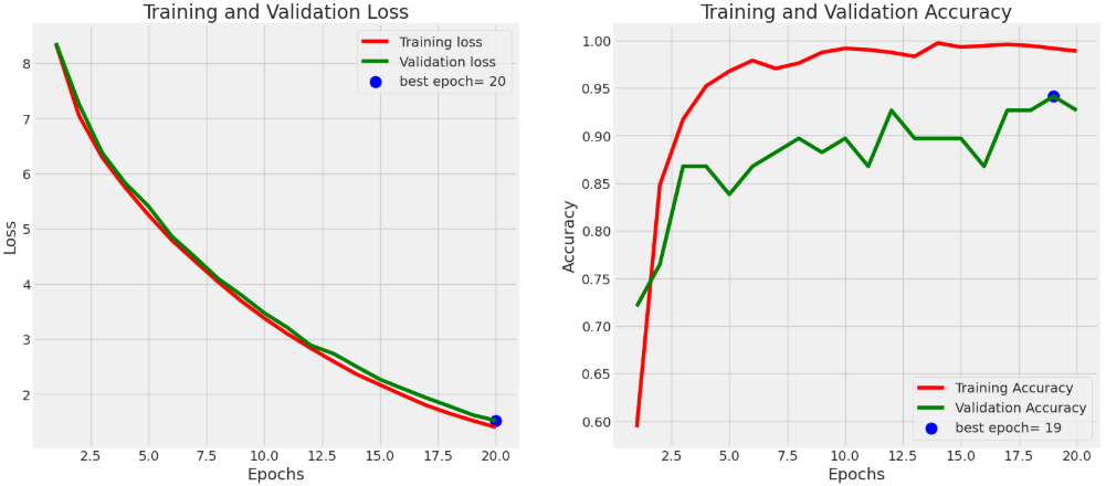

2. 多数据集定量评估

为了客观评估模型的泛化性能，代码根据测试集样本总量动态计算最佳评估 Batch Size 与评估步数（steps），随后分别对训练集、验证集与测试集执行评分计算，并输出直观的数值结果。

# ----------------------------------------------------------------------
# 1. 动态计算适配测试集样本数的 Batch Size 与 Steps
# ----------------------------------------------------------------------
ts_length = len(test_df)
test_batch_size = max(sorted([ts_length // n for n in range(1, ts_length + 1) if ts_length%n == 0 and ts_length/n <= 80]))
test_steps = ts_length // test_batch_size
# ----------------------------------------------------------------------
# 2. 分别评估训练集、验证集与测试集指标
# ----------------------------------------------------------------------
train_score = model.evaluate(train_gen, steps= test_steps, verbose= 1)
valid_score = model.evaluate(valid_gen, steps= test_steps, verbose= 1)
test_score = model.evaluate(test_gen, steps= test_steps, verbose= 1)
# ----------------------------------------------------------------------
# 3. 打印输出各集合损失与准确率
# ----------------------------------------------------------------------
print("Train Loss: ", train_score[0])
print("Train Accuracy: ", train_score[1])
print('-' * 20)
print("Validation Loss: ", valid_score[0])
print("Validation Accuracy: ", valid_score[1])
print('-' * 20)
print("Test Loss: ", test_score[0])
print("Test Accuracy: ", test_score[1])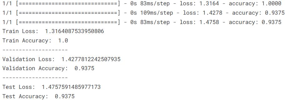

3. 混淆矩阵分析

利用测试集生成器获取预测概率矩阵并提取概率最大的类别索引，计算真实标签与预测标签之间的混淆矩阵，以热力图的形式生动呈现各个鞋类品牌之间的交叉误判细节。

# ----------------------------------------------------------------------
# 1. 获取测试集预测结果与类别映射
# ----------------------------------------------------------------------
preds = model.predict_generator(test_gen)
y_pred = np.argmax(preds, axis=1)
g_dict = test_gen.class_indices
classes = list(g_dict.keys())
# ----------------------------------------------------------------------
# 2. 计算并绘制混淆矩阵热力图
# ----------------------------------------------------------------------
cm = confusion_matrix(test_gen.classes, y_pred)
plt.figure(figsize= (10, 10))
plt.imshow(cm, interpolation= 'nearest', cmap= plt.cm.Blues)
plt.title('Confusion Matrix')
plt.colorbar()
tick_marks = np.arange(len(classes))
plt.xticks(tick_marks, classes, rotation= 45)
plt.yticks(tick_marks, classes)
# 在热力图中添加具体数值文本标签，并根据数值深浅自动调整字体颜色
thresh = cm.max() / 2.
for i, j in itertools.product(range(cm.shape[0]), range(cm.shape[1])):
    plt.text(j, i, cm[i, j], horizontalalignment= 'center', color= 'white' if cm[i, j] > thresh else 'black')
plt.tight_layout()
plt.ylabel('True Label')
plt.xlabel('Predicted Label')
plt.show()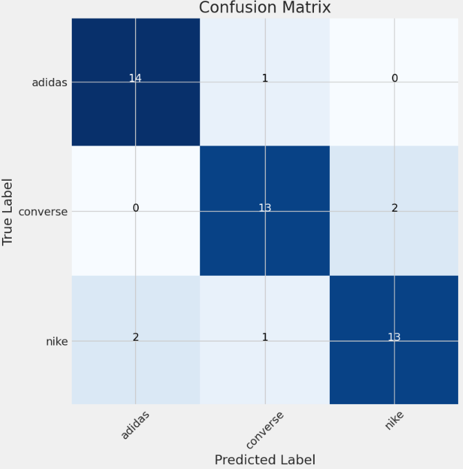

4. 分类性能综合报告

最后调用 classification_report 函数打印测试集分类性能报告，细化输出每个鞋类品牌类别的 Precision、Recall、F1-Score 以及全局的 Macro Average 与 Weighted Average 指标。

# ----------------------------------------------------------------------
# 输出详细的分类性能评估报告
# ----------------------------------------------------------------------
print(classification_report(test_gen.classes, y_pred, target_names= classes))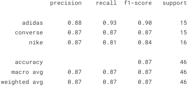

最后可以保存模型

#Save the model
model.save('model.h5')

5.总结

本实验基于包含阿迪达斯、匡威及耐克三个品牌图像的鞋类分类数据集，构建了基于 EfficientNetB0 迁移学习架构的图像识别模型。数据集由 711 张训练图像与 114 张测试图像组成，图像尺寸统一调整为 224×224 像素的 RGB 三通道输入。通过在预训练主干网络上叠加 BatchNormalization、带 L1/L2 正则化的全连接层以及 Dropout 结构，模型在 20 轮迭代中展现出了平稳的收敛性能。最终评估结果表明，模型在训练集上达到了 100% 的准确率，在验证集与测试集上的评估准确率均保持在 93.75%，并在最终的测试集独立评估中取得了 87% 的综合分类准确率与 F1 分数。整体而言，该模型对于三种鞋类品牌具备优秀的特征提取能力与泛化识别性能，验证了预训练卷积神经网络结合多重正则化策略在小样本多分类任务中的有效性与实用价值。

源代码

# import system libs
import os
import time
import shutil
import pathlib
import itertools
from PIL import Image
# import data handling tools
import cv2
import numpy as np
import pandas as pd
import seaborn as sns
sns.set_style('darkgrid')
import matplotlib.pyplot as plt
from sklearn.model_selection import train_test_split
from sklearn.metrics import confusion_matrix, classification_report
# import Deep learning Libraries
import tensorflow as tf
from tensorflow import keras
from tensorflow.keras.models import Sequential
from tensorflow.keras.optimizers import Adam, Adamax
from tensorflow.keras.metrics import categorical_crossentropy
from tensorflow.keras.preprocessing.image import ImageDataGenerator
from tensorflow.keras.layers import Conv2D, MaxPooling2D, Flatten, Dense, Activation, Dropout, BatchNormalization
from tensorflow.keras import regularizers
# Ignore Warnings
import warnings
warnings.filterwarnings("ignore")
train_dir = '/kaggle/input/nike-adidas-and-converse-imaged/train'
filepaths = []
labels = []

folds = os.listdir(train_dir)
for fold in folds:
    foldpath = os.path.join(train_dir, fold)
    filelist = os.listdir(foldpath)
    for file in filelist:
        fpath = os.path.join(foldpath, file)
        filepaths.append(fpath)
        labels.append(fold)

# Concatenate data paths with labels into one dataframe
Fseries = pd.Series(filepaths, name= 'filepaths')
Lseries = pd.Series(labels, name='labels')
train_df = pd.concat([Fseries, Lseries], axis= 1)
# Generate  test data paths with labels
test_dir = '/kaggle/input/nike-adidas-and-converse-imaged/test'
filepaths = []
labels = []

folds = os.listdir(test_dir)
for fold in folds:
    foldpath = os.path.join(test_dir, fold)
    filelist = os.listdir(foldpath)
    for file in filelist:
        fpath = os.path.join(foldpath, file)
        filepaths.append(fpath)
        labels.append(fold)

# Concatenate data paths with labels into one dataframe
Fseries = pd.Series(filepaths, name= 'filepaths')
Lseries = pd.Series(labels, name='labels')
test_df = pd.concat([Fseries, Lseries], axis= 1)
test_df
# valid and test dataframe
valid_df, test_df = train_test_split(test_df,  train_size= 0.6, shuffle= True, random_state= 123)
# crobed image size
batch_size = 16
img_size = (224, 224)
channels = 3
img_shape = (img_size[0], img_size[1], channels)

tr_gen = ImageDataGenerator()
ts_gen = ImageDataGenerator()
train_gen = tr_gen.flow_from_dataframe( train_df, x_col= 'filepaths', y_col= 'labels', target_size= img_size, class_mode= 'categorical',
                                    color_mode= 'rgb', shuffle= True, batch_size= batch_size)

valid_gen = ts_gen.flow_from_dataframe( valid_df, x_col= 'filepaths', y_col= 'labels', target_size= img_size, class_mode= 'categorical',
                                    color_mode= 'rgb', shuffle= True, batch_size= batch_size)

test_gen = ts_gen.flow_from_dataframe( test_df, x_col= 'filepaths', y_col= 'labels', target_size= img_size, class_mode= 'categorical',
                                    color_mode= 'rgb', shuffle= False, batch_size= batch_size)
g_dict = train_gen.class_indices      # defines dictionary {'class': index}
classes = list(g_dict.keys())       # defines list of dictionary's kays (classes), classes names : string
images, labels = next(train_gen)      # get a batch size samples from the generator

plt.figure(figsize= (20, 20))

for i in range(16):
    plt.subplot(4, 4, i + 1)
    image = images[i] / 255       # scales data to range (0 - 255)
    plt.imshow(image)
    index = np.argmax(labels[i])  # get image index
    class_name = classes[index]   # get class of image
    plt.title(class_name, color= 'blue', fontsize= 12)
    plt.axis('off')
plt.show()
# Create Model Structure
img_size = (224, 224)
channels = 3
img_shape = (img_size[0], img_size[1], channels)
class_count = len(list(train_gen.class_indices.keys())) # to define number of classes in dense layer

# create pre-trained model (you can built on pretrained model such as :  efficientnet, VGG , Resnet )
# we will use efficientnetb3 from EfficientNet family.
base_model = tf.keras.applications.efficientnet.EfficientNetB0(include_top= False, weights= "imagenet", input_shape= img_shape, pooling= 'max')
# base_model.trainable = False
model = Sequential([
    base_model,
    BatchNormalization(axis= -1, momentum= 0.99, epsilon= 0.001),
    Dense(256, kernel_regularizer= regularizers.l2(l= 0.016), activity_regularizer= regularizers.l1(0.006),
                bias_regularizer= regularizers.l1(0.006), activation= 'relu'),
    Dropout(rate= 0.45, seed= 123),
    Dense(class_count, activation= 'softmax')
])

model.compile(Adamax(learning_rate= 0.001), loss= 'categorical_crossentropy', metrics= ['accuracy'])

model.summary()
batch_size = 20   # set batch size for training
epochs =  20  # number of all epochs in training

history = model.fit(x= train_gen, epochs= epochs, verbose= 1, validation_data= valid_gen, 
                    validation_steps= None, shuffle= False)
# Define needed variables
tr_acc = history.history['accuracy']
tr_loss = history.history['loss']
val_acc = history.history['val_accuracy']
val_loss = history.history['val_loss']
index_loss = np.argmin(val_loss)
val_lowest = val_loss[index_loss]
index_acc = np.argmax(val_acc)
acc_highest = val_acc[index_acc]
Epochs = [i+1 for i in range(len(tr_acc))]
loss_label = f'best epoch= {str(index_loss + 1)}'
acc_label = f'best epoch= {str(index_acc + 1)}'
# Plot training history
plt.figure(figsize= (20, 8))
plt.style.use('fivethirtyeight')
plt.subplot(1, 2, 1)
plt.plot(Epochs, tr_loss, 'r', label= 'Training loss')
plt.plot(Epochs, val_loss, 'g', label= 'Validation loss')
plt.scatter(index_loss + 1, val_lowest, s= 150, c= 'blue', label= loss_label)
plt.title('Training and Validation Loss')
plt.xlabel('Epochs')
plt.ylabel('Loss')
plt.legend()
plt.subplot(1, 2, 2)
plt.plot(Epochs, tr_acc, 'r', label= 'Training Accuracy')
plt.plot(Epochs, val_acc, 'g', label= 'Validation Accuracy')
plt.scatter(index_acc + 1 , acc_highest, s= 150, c= 'blue', label= acc_label)
plt.title('Training and Validation Accuracy')
plt.xlabel('Epochs')
plt.ylabel('Accuracy')
plt.legend()
plt.tight_layout
plt.show()
ts_length = len(test_df)
test_batch_size = max(sorted([ts_length // n for n in range(1, ts_length + 1) if ts_length%n == 0 and ts_length/n <= 80]))
test_steps = ts_length // test_batch_size

train_score = model.evaluate(train_gen, steps= test_steps, verbose= 1)
valid_score = model.evaluate(valid_gen, steps= test_steps, verbose= 1)
test_score = model.evaluate(test_gen, steps= test_steps, verbose= 1)

print("Train Loss: ", train_score[0])
print("Train Accuracy: ", train_score[1])
print('-' * 20)
print("Validation Loss: ", valid_score[0])
print("Validation Accuracy: ", valid_score[1])
print('-' * 20)
print("Test Loss: ", test_score[0])
print("Test Accuracy: ", test_score[1])
preds = model.predict_generator(test_gen)
y_pred = np.argmax(preds, axis=1)
g_dict = test_gen.class_indices
classes = list(g_dict.keys())

# Confusion matrix
cm = confusion_matrix(test_gen.classes, y_pred)

plt.figure(figsize= (10, 10))
plt.imshow(cm, interpolation= 'nearest', cmap= plt.cm.Blues)
plt.title('Confusion Matrix')
plt.colorbar()

tick_marks = np.arange(len(classes))
plt.xticks(tick_marks, classes, rotation= 45)
plt.yticks(tick_marks, classes)
thresh = cm.max() / 2.
for i, j in itertools.product(range(cm.shape[0]), range(cm.shape[1])):
    plt.text(j, i, cm[i, j], horizontalalignment= 'center', color= 'white' if cm[i, j] > thresh else 'black')

plt.tight_layout()
plt.ylabel('True Label')
plt.xlabel('Predicted Label')

plt.show()
# Classification report
print(classification_report(test_gen.classes, y_pred, target_names= classes))

资料获取，更多粉丝福利，关注下方公众号获取