R语言绘图 --- 气泡图（Biorplot 开发日志 --- 4）

「写在前面」

在科研数据分析中我们会重复地绘制一些图形，如果代码管理不当经常就会忘记之前绘图的代码。于是我计划开发一个 R 包（Biorplot），用来管理自己 R 语言绘图的代码。本系列文章用于记录 Biorplot 包开发日志。

介绍

气泡图，是一种以二维图形展示多维数据的可视化工具。它将数据点绘制在平面坐标系中，每个数据点用一个圆圈表示，圆圈的大小通常与某个维度的数值大小相关。通过气泡图，我们可以轻松地观察到数据点在各个维度上的分布情况，从而更好地理解数据的结构和规律。

在 Biorplot 中，我封装了 Bior_DotPlot() 函数来实现气泡图的绘制。

基础气泡图

绘制一个基础的气泡图如下：

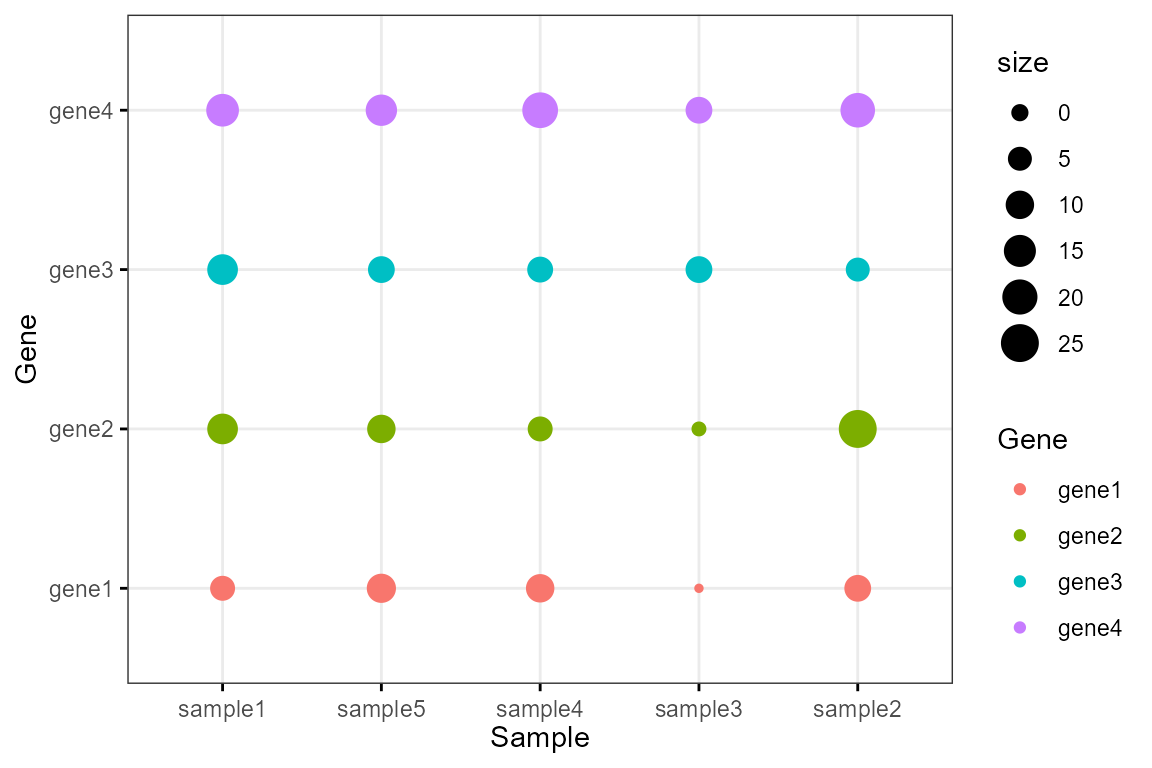
绘图代码：

df <- data.frame(
  Sample = rep(paste('sample', 1:5, sep=''), 4),
  Gene = rep(paste('gene', 1:4, sep=''), 5),
  size = round(rnorm(20, mean = 10, sd = 5))
)
colour <- c("#1F77B4FF","#FF7F0EFF","#2CA02CFF","#D62728FF","#9467BDFF")
Bior_DotPlot(data = df, x = "Sample", y = "Gene", size = "size", color = "Gene",
             x.text.col = F, ggtheme = theme_bw()) + 
  theme(axis.text.x = element_text(angle = 0, hjust = 0.5))

表达量气泡图

绘制一个表达量气泡图如下：

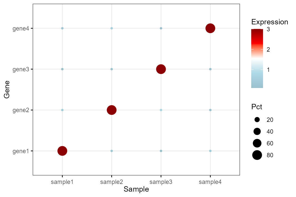
绘图代码：

df <- data.frame(
  Sample = rep(paste('sample', 1:4, sep=''), each=4),
  Gene = rep(paste('gene', 1:4, sep=''), 4),
  Pct = c(80,10,10,10,10,80,10,10,10,10,80,10,10,10,10,80),
  Expression = c(3,0.5,0.1,0.3,0.3,3,0.2,0.6,0.1,0.7,3,0.1,0.5,0.2,0.1,3)
)

Bior_DotPlot(data = df, x = "Sample", y = "Gene", size="Pct", color = "Expression",
             x.text.col = F, ggtheme = theme_bw()) + 
  theme(axis.text.x = element_text(angle = 0, hjust = 0.5)) +
  scale_color_gradientn(colours = c("lightblue3", "lightblue", "white", "red", "red4"))

源码解析

Biorplot::Bior_DotPlot() 函数主要继承了 ggpubr::ggdotchart() 函数。

源码：

#%%%%%%%%%%%%%%%%%%%%%%%%%%%%%%%%%%%%%%%%%%%%%%%%%%%%%%%%%%%%%%%%%%%%%%%%%%%%%%%

#' Dot Plot
#' @description Create a dot plot.
#'
#' @importFrom ggpubr ggdotchart
#' @import ggplot2
#'
#' @inheritParams ggpubr::ggdotchart
#'
#' @return A ggplot object
#' @export
#'
#' @examples
#' # Examples 1
#' x <- rep(paste('sample', 1:5, sep=''), 4)
#' y <- rep(paste('gene', 1:4, sep=''), 5)
#' size <- round(rnorm(20, mean = 10, sd = 5))
#' colour <- c("#1F77B4FF","#FF7F0EFF","#2CA02CFF","#D62728FF","#9467BDFF")
#' p <- Bior_DotPlot(x = x, y = y, size = size, group.by = x, colour = colour, max_size=10)
#' p
Bior_DotPlot <- function(data, x, y, group = NULL,
                         combine = FALSE,
                         color = "black", palette = NULL,
                         shape = 19, size = NULL, dot.size = size,
                         sorting = c("ascending", "descending", "none"),
                         x.text.col = TRUE,
                         rotate = FALSE,
                         title = NULL, xlab = NULL, ylab = NULL,
                         facet.by = NULL, panel.labs = NULL, short.panel.labs = TRUE,
                         select = NULL, remove = NULL, order = NULL,
                         label = NULL, font.label = list(size = 11, color = "black"),
                         label.select = NULL, repel = FALSE, label.rectangle = FALSE,
                         position = "identity",
                         ggtheme = theme_pubr(),
                         ...)
{
  # Default options
  .opts <- list(data = data, x = x, y = y, group = group,
                combine = combine,
                color = color, palette = palette,
                shape = shape, size = size, dot.size = size,
                sorting = sorting,
                x.text.col = x.text.col,
                rotate = rotate,
                title = title, xlab = xlab, ylab = ylab,
                facet.by = facet.by, panel.labs = panel.labs, short.panel.labs = short.panel.labs,
                select = select, remove = remove, order = order,
                label = label, font.label = font.label,
                label.select = label.select, repel = repel, label.rectangle = label.rectangle,
                position = position,
                ggtheme = ggtheme,
                ...)

  p <- do.call(ggpubr::ggdotchart, .opts)

  return(p)
}

#%%%%%%%%%%%%%%%%%%%%%%%%%%%%%%%%%%%%%%%%%%%%%%%%%%%%%%%%%%%%%%%%%%%%%%%%%%%%%%%

「结束」

注：本文为个人学习笔记，仅供大家参考学习，不得用于任何商业目的。如有侵权，请联系作者删除。

本文由mdnice多平台发布

R语言绘图 --- 气泡图（Biorplot 开发日志 --- 4）

「写在前面」

相关链接

介绍

基础气泡图

表达量气泡图

源码解析