- 🍨 本文为🔗365天深度学习训练营 中的学习记录博客
- 🍖 原作者:K同学啊
前期准备工作
python
import torch.nn.functional as F
import numpy as np
import pandas as pd
import torch
from torch import nn
1. 导入数据
python
data = pd.read_csv(r"D:\Personal Data\Learning Data\DL Learning Data\LSTM\woodpine2.csv")
data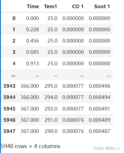
2. 数据可视化
python
import matplotlib.pyplot as plt
import seaborn as sns

plt.rcParams['savefig.dpi'] = 500 #图片像素
plt.rcParams['figure.dpi'] = 500 #分辨率
fig, ax = plt.subplots(1,3,constrained_layout = True, figsize = (14, 3))

sns.lineplot(data = data["Tem1"], ax = ax[0])
sns.lineplot(data=data['CO 1'], ax = ax[1])
sns.lineplot(data=data["Soot 1"], ax = ax[2])
plt.show()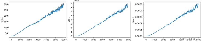
python
dataFrame = data.iloc[:,1:]
dataFrame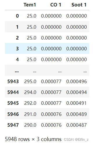
二、构建数据集
1. 数据集预处理
python
from sklearn.preprocessing import MinMaxScaler

dataFrame = data.iloc[:,1:].copy()
sc = MinMaxScaler(feature_range=(0,1))   #将数据归一化
for i in ['CO 1', 'Soot 1', 'Tem1']:
    dataFrame[i] = sc.fit_transform(dataFrame[i].values.reshape(-1,1))

dataFrame.shape
输出:
python
(5948, 3)2. 设置X、y
python
width_X = 8
width_y = 1

## 取前8个时间段的Tem1、CO 1、Soot 1为X,第9个时间段的Tem1为y。
X = []
y = []

in_start = 0
for _,_ in data.iterrows():
    in_end = in_start + width_X
    out_end = in_end + width_y

    if out_end < len(dataFrame):
        X_ = np.array(dataFrame.iloc[in_start:in_end, ])
        y_ = np.array(dataFrame.iloc[in_end: out_end, 0])

        X.append(X_)
        y.append(y_)
    in_start += 1

X = np.array(X)
y = np.array(y).reshape(-1,1,1)
X.shape, y.shape
输出:
python
((5939, 8, 3), (5939, 1, 1))检查数据集是否有空值
python
#检查数据集是否有空值
print(np.any(np.isnan(X)))
print(np.any(np.isnan(y)))
3. 划分数据集
python
X_train = torch.tensor(np.array(X[:5000]), dtype=torch.float32)
y_train = torch.tensor(np.array(y[:5000]), dtype=torch.float32)

X_test  = torch.tensor(np.array(X[5000:]), dtype=torch.float32)
y_test  = torch.tensor(np.array(y[5000:]), dtype=torch.float32)
X_train.shape, y_train.shape
输出:
python
(torch.Size([5000, 8, 3]), torch.Size([5000, 1, 1]))
python
from torch.utils.data import TensorDataset, DataLoader
train_dl = DataLoader(TensorDataset(X_train, y_train),
                      batch_size=64,
                      shuffle=False)
test_dl = DataLoader(TensorDataset(X_test, y_test),
                     batch_size=64,
                     shuffle=False)
三、模型训练
1. 构建模型
python
class model_lstm(nn.Module):
    def __init__(self):
        super(model_lstm, self).__init__()
        self.lstm0 = nn.LSTM(input_size=3 ,hidden_size=320,
                             num_layers=1, batch_first=True)
        self.lstm1 = nn.LSTM(input_size=320 ,hidden_size=320,
                             num_layers=1, batch_first=True)
        self.fc0 = nn.Linear(320, 1)
        # self.fc1 = nn.Sequential(nn.Linear(300, 2))

    def forward(self, x):
        #如果不传入h0和c0,pytorch会将其初始化为0
        out, hidden1 = self.lstm0(x)
        out, _ = self.lstm1(out, hidden1)
        out = self.fc0(out)
        return out[:, -1:, :]   #取2个预测值,否则经过lstm会得到8*2个预测
model = model_lstm()
model
输出:
python
model_lstm(
  (lstm0): LSTM(3, 320, batch_first=True)
  (lstm1): LSTM(320, 320, batch_first=True)
  (fc0): Linear(in_features=320, out_features=1, bias=True)
)
python
model(torch.rand(30,8,3)).shape输出:
python
torch.Size([30, 1, 1])2.定义训练函数
python
# 训练循环
import copy
def train(train_dl, model, loss_fn, opt, lr_scheduler=None):
    size = len(train_dl.dataset)
    num_batches = len(train_dl)
    train_loss = 0  # 初始化训练损失和正确率

    for x, y in train_dl:
        x, y = x.to(device), y.to(device)

        # 计算预测误差
        #pred = model(x)
        pred = model(x)          # 网络输出
        loss = loss_fn(pred, y)  # 计算网络输出和真实值之间的差距

        # 反向传播
        opt.zero_grad()  # grad属性归零
        loss.backward()        # 反向传播
        opt.step()       # 每一步自动更新

        # 记录loss
        train_loss += loss.item()
    if lr_scheduler is not None:
        lr_scheduler.step()
        print("learning rate = ", opt.param_groups[0]['lr'])
    train_loss /= num_batches
    return train_loss
3. 定义测试函数
python
def test (dataloader, model, loss_fn):
    size        = len(dataloader.dataset)  # 测试集的大小
    num_batches = len(dataloader)          # 批次数目
    test_loss = 0

    # 当不进行训练时,停止梯度更新,节省计算内存消耗
    with torch.no_grad():
        for x, y in dataloader:

            x, y = x.to(device), y.to(device)

            # 计算loss
            y_pred = model(x)
            loss        = loss_fn(y_pred, y)
            test_loss += loss.item()

    test_loss /= num_batches
    return test_loss
4. 正式训练模型
python
#设置GPU训练
import torch
device=torch.device("cuda" if torch.cuda.is_available() else "cpu")
device
输出:
python
device(type='cuda')
python
#训练模型
model = model_lstm()
model = model.to(device)
loss_fn    = nn.MSELoss() # 创建损失函数
learn_rate = 1e-1   # 学习率
opt        = torch.optim.SGD(model.parameters(),lr=learn_rate,weight_decay=1e-4)
epochs     = 150
train_loss = []
test_loss  = []
lr_scheduler = torch.optim.lr_scheduler.CosineAnnealingLR(opt,epochs, last_epoch=-1)
best_val =[0, 1e5]
for epoch in range(epochs):
    model.train()
    epoch_train_loss = train(train_dl, model, loss_fn, opt, lr_scheduler)

    model.eval()
    epoch_test_loss = test(test_dl, model, loss_fn)
    if best_val[1] >  epoch_test_loss:
        best_val =[epoch, epoch_test_loss]
        best_model_wst = copy.deepcopy(model.state_dict())

    train_loss.append(epoch_train_loss)
    test_loss.append(epoch_test_loss)

    template = ('Epoch:{:2d}, Train_loss:{:.6f}, Test_loss:{:.6f}')
    print(template.format(epoch+1, epoch_train_loss,  epoch_test_loss))
print("*"*20, 'Done', "*"*20)
输出:
python
learning rate =  0.09998903417374227
Epoch: 1, Train_loss:0.001263, Test_loss:0.012446
learning rate =  0.09995614150494292
Epoch: 2, Train_loss:0.014234, Test_loss:0.012052
learning rate =  0.09990133642141358
Epoch: 3, Train_loss:0.013899, Test_loss:0.011644
learning rate =  0.09982464296247522
Epoch: 4, Train_loss:0.013514, Test_loss:0.011209
learning rate =  0.09972609476841367
Epoch: 5, Train_loss:0.013065, Test_loss:0.010731
learning rate =  0.0996057350657239
Epoch: 6, Train_loss:0.012539, Test_loss:0.010204
learning rate =  0.09946361664814941
Epoch: 7, Train_loss:0.011923, Test_loss:0.009617
learning rate =  0.09929980185352524
Epoch: 8, Train_loss:0.011208, Test_loss:0.008970
learning rate =  0.09911436253643444
Epoch: 9, Train_loss:0.010392, Test_loss:0.008263
learning rate =  0.09890738003669028
Epoch:10, Train_loss:0.009476, Test_loss:0.007508
learning rate =  0.098678945143658
Epoch:11, Train_loss:0.008475, Test_loss:0.006716
learning rate =  0.09842915805643156
Epoch:12, Train_loss:0.007412, Test_loss:0.005910
learning rate =  0.09815812833988291
Epoch:13, Train_loss:0.006323, Test_loss:0.005112
learning rate =  0.09786597487660335
Epoch:14, Train_loss:0.005249, Test_loss:0.004352
learning rate =  0.09755282581475769
Epoch:15, Train_loss:0.004237, Test_loss:0.003654
learning rate =  0.09721881851187407
Epoch:16, Train_loss:0.003325, Test_loss:0.003036
learning rate =  0.0968640994745946
Epoch:17, Train_loss:0.002540, Test_loss:0.002509
learning rate =  0.09648882429441258
Epoch:18, Train_loss:0.001895, Test_loss:0.002082
learning rate =  0.09609315757942503
Epoch:19, Train_loss:0.001388, Test_loss:0.001740
learning rate =  0.09567727288213004
Epoch:20, Train_loss:0.001005, Test_loss:0.001479
learning rate =  0.09524135262330098
Epoch:21, Train_loss:0.000725, Test_loss:0.001283
learning rate =  0.09478558801197065
Epoch:22, Train_loss:0.000526, Test_loss:0.001138
learning rate =  0.09431017896156073
Epoch:23, Train_loss:0.000388, Test_loss:0.001033
learning rate =  0.09381533400219318
Epoch:24, Train_loss:0.000294, Test_loss:0.000955
learning rate =  0.09330127018922194
Epoch:25, Train_loss:0.000230, Test_loss:0.000900
learning rate =  0.09276821300802535
Epoch:26, Train_loss:0.000188, Test_loss:0.000859
learning rate =  0.09221639627510077
Epoch:27, Train_loss:0.000159, Test_loss:0.000829
learning rate =  0.09164606203550499
Epoch:28, Train_loss:0.000139, Test_loss:0.000806
learning rate =  0.09105746045668521
Epoch:29, Train_loss:0.000126, Test_loss:0.000789
learning rate =  0.09045084971874738
Epoch:30, Train_loss:0.000117, Test_loss:0.000775
learning rate =  0.08982649590120982
Epoch:31, Train_loss:0.000110, Test_loss:0.000765
learning rate =  0.089184672866292
Epoch:32, Train_loss:0.000105, Test_loss:0.000755
learning rate =  0.08852566213878947
Epoch:33, Train_loss:0.000102, Test_loss:0.000749
learning rate =  0.08784975278258783
Epoch:34, Train_loss:0.000100, Test_loss:0.000743
learning rate =  0.08715724127386973
Epoch:35, Train_loss:0.000098, Test_loss:0.000738
learning rate =  0.08644843137107058
Epoch:36, Train_loss:0.000096, Test_loss:0.000731
learning rate =  0.08572363398164018
Epoch:37, Train_loss:0.000095, Test_loss:0.000727
learning rate =  0.0849831670256683
Epoch:38, Train_loss:0.000094, Test_loss:0.000724
learning rate =  0.08422735529643445
Epoch:39, Train_loss:0.000094, Test_loss:0.000720
learning rate =  0.08345653031794292
Epoch:40, Train_loss:0.000093, Test_loss:0.000717
learning rate =  0.0826710301995053
Epoch:41, Train_loss:0.000093, Test_loss:0.000712
learning rate =  0.0818711994874345
Epoch:42, Train_loss:0.000092, Test_loss:0.000708
learning rate =  0.08105738901391554
Epoch:43, Train_loss:0.000092, Test_loss:0.000705
learning rate =  0.08022995574311877
Epoch:44, Train_loss:0.000092, Test_loss:0.000701
learning rate =  0.07938926261462367
Epoch:45, Train_loss:0.000092, Test_loss:0.000698
learning rate =  0.07853567838422161
Epoch:46, Train_loss:0.000091, Test_loss:0.000694
learning rate =  0.07766957746216722
Epoch:47, Train_loss:0.000091, Test_loss:0.000692
learning rate =  0.07679133974894985
Epoch:48, Train_loss:0.000091, Test_loss:0.000688
learning rate =  0.07590135046865654
Epoch:49, Train_loss:0.000091, Test_loss:0.000683
learning rate =  0.07500000000000002
Epoch:50, Train_loss:0.000091, Test_loss:0.000681
learning rate =  0.07408768370508578
Epoch:51, Train_loss:0.000091, Test_loss:0.000676
learning rate =  0.07316480175599312
Epoch:52, Train_loss:0.000090, Test_loss:0.000672
learning rate =  0.0722317589592464
Epoch:53, Train_loss:0.000090, Test_loss:0.000668
learning rate =  0.07128896457825366
Epoch:54, Train_loss:0.000090, Test_loss:0.000666
learning rate =  0.07033683215379004
Epoch:55, Train_loss:0.000090, Test_loss:0.000662
learning rate =  0.06937577932260518
Epoch:56, Train_loss:0.000090, Test_loss:0.000658
learning rate =  0.06840622763423394
Epoch:57, Train_loss:0.000090, Test_loss:0.000654
learning rate =  0.0674286023660908
Epoch:58, Train_loss:0.000090, Test_loss:0.000650
learning rate =  0.0664433323369292
Epoch:59, Train_loss:0.000090, Test_loss:0.000646
learning rate =  0.06545084971874741
Epoch:60, Train_loss:0.000090, Test_loss:0.000643
learning rate =  0.06445158984722361
Epoch:61, Train_loss:0.000090, Test_loss:0.000639
learning rate =  0.06344599103076332
Epoch:62, Train_loss:0.000090, Test_loss:0.000635
learning rate =  0.06243449435824276
Epoch:63, Train_loss:0.000089, Test_loss:0.000631
learning rate =  0.06141754350553282
Epoch:64, Train_loss:0.000089, Test_loss:0.000627
learning rate =  0.060395584540888
Epoch:65, Train_loss:0.000089, Test_loss:0.000623
learning rate =  0.05936906572928627
Epoch:66, Train_loss:0.000089, Test_loss:0.000620
learning rate =  0.05833843733580514
Epoch:67, Train_loss:0.000089, Test_loss:0.000615
learning rate =  0.05730415142812061
Epoch:68, Train_loss:0.000089, Test_loss:0.000612
learning rate =  0.056266661678215237
Epoch:69, Train_loss:0.000089, Test_loss:0.000608
learning rate =  0.055226423163382714
Epoch:70, Train_loss:0.000089, Test_loss:0.000604
learning rate =  0.0541838921666158
Epoch:71, Train_loss:0.000089, Test_loss:0.000601
learning rate =  0.0531395259764657
Epoch:72, Train_loss:0.000090, Test_loss:0.000597
learning rate =  0.05209378268646001
Epoch:73, Train_loss:0.000090, Test_loss:0.000593
learning rate =  0.051047120994167874
Epoch:74, Train_loss:0.000090, Test_loss:0.000590
learning rate =  0.050000000000000024
Epoch:75, Train_loss:0.000090, Test_loss:0.000587
learning rate =  0.048952879005832194
Epoch:76, Train_loss:0.000090, Test_loss:0.000583
learning rate =  0.04790621731354004
Epoch:77, Train_loss:0.000090, Test_loss:0.000579
learning rate =  0.04686047402353437
Epoch:78, Train_loss:0.000090, Test_loss:0.000576
learning rate =  0.045816107833384245
Epoch:79, Train_loss:0.000090, Test_loss:0.000573
learning rate =  0.044773576836617354
Epoch:80, Train_loss:0.000091, Test_loss:0.000569
learning rate =  0.04373333832178481
Epoch:81, Train_loss:0.000091, Test_loss:0.000567
learning rate =  0.042695848571879455
Epoch:82, Train_loss:0.000091, Test_loss:0.000563
learning rate =  0.0416615626641949
Epoch:83, Train_loss:0.000091, Test_loss:0.000561
learning rate =  0.040630934270713785
Epoch:84, Train_loss:0.000091, Test_loss:0.000558
learning rate =  0.039604415459112044
Epoch:85, Train_loss:0.000092, Test_loss:0.000555
learning rate =  0.03858245649446723
Epoch:86, Train_loss:0.000092, Test_loss:0.000552
learning rate =  0.03756550564175728
Epoch:87, Train_loss:0.000092, Test_loss:0.000550
learning rate =  0.03655400896923674
Epoch:88, Train_loss:0.000093, Test_loss:0.000548
learning rate =  0.03554841015277642
Epoch:89, Train_loss:0.000093, Test_loss:0.000545
learning rate =  0.03454915028125264
Epoch:90, Train_loss:0.000094, Test_loss:0.000543
learning rate =  0.03355666766307085
Epoch:91, Train_loss:0.000094, Test_loss:0.000541
learning rate =  0.03257139763390926
Epoch:92, Train_loss:0.000095, Test_loss:0.000539
learning rate =  0.031593772365766125
Epoch:93, Train_loss:0.000095, Test_loss:0.000538
learning rate =  0.030624220677394863
Epoch:94, Train_loss:0.000096, Test_loss:0.000536
learning rate =  0.02966316784621
Epoch:95, Train_loss:0.000096, Test_loss:0.000535
learning rate =  0.02871103542174638
Epoch:96, Train_loss:0.000097, Test_loss:0.000534
learning rate =  0.02776824104075365
Epoch:97, Train_loss:0.000098, Test_loss:0.000533
learning rate =  0.026835198244006937
Epoch:98, Train_loss:0.000098, Test_loss:0.000532
learning rate =  0.02591231629491424
Epoch:99, Train_loss:0.000099, Test_loss:0.000531
learning rate =  0.024999999999999998
Epoch:100, Train_loss:0.000100, Test_loss:0.000531
learning rate =  0.024098649531343507
Epoch:101, Train_loss:0.000101, Test_loss:0.000530
learning rate =  0.023208660251050187
Epoch:102, Train_loss:0.000102, Test_loss:0.000530
learning rate =  0.02233042253783281
Epoch:103, Train_loss:0.000103, Test_loss:0.000530
learning rate =  0.021464321615778426
Epoch:104, Train_loss:0.000104, Test_loss:0.000530
learning rate =  0.020610737385376356
Epoch:105, Train_loss:0.000105, Test_loss:0.000531
learning rate =  0.019770044256881267
Epoch:106, Train_loss:0.000106, Test_loss:0.000531
learning rate =  0.018942610986084494
Epoch:107, Train_loss:0.000107, Test_loss:0.000532
learning rate =  0.018128800512565522
Epoch:108, Train_loss:0.000108, Test_loss:0.000533
learning rate =  0.01732896980049475
Epoch:109, Train_loss:0.000110, Test_loss:0.000535
learning rate =  0.016543469682057093
Epoch:110, Train_loss:0.000111, Test_loss:0.000536
learning rate =  0.01577264470356557
Epoch:111, Train_loss:0.000112, Test_loss:0.000537
learning rate =  0.015016832974331734
Epoch:112, Train_loss:0.000113, Test_loss:0.000539
learning rate =  0.014276366018359849
Epoch:113, Train_loss:0.000115, Test_loss:0.000541
learning rate =  0.01355156862892944
Epoch:114, Train_loss:0.000116, Test_loss:0.000544
learning rate =  0.012842758726130289
Epoch:115, Train_loss:0.000118, Test_loss:0.000546
learning rate =  0.012150247217412192
Epoch:116, Train_loss:0.000119, Test_loss:0.000549
learning rate =  0.011474337861210548
Epoch:117, Train_loss:0.000120, Test_loss:0.000552
learning rate =  0.010815327133708018
Epoch:118, Train_loss:0.000122, Test_loss:0.000555
learning rate =  0.010173504098790198
Epoch:119, Train_loss:0.000123, Test_loss:0.000557
learning rate =  0.009549150281252639
Epoch:120, Train_loss:0.000124, Test_loss:0.000561
learning rate =  0.008942539543314802
Epoch:121, Train_loss:0.000126, Test_loss:0.000564
learning rate =  0.008353937964495033
Epoch:122, Train_loss:0.000127, Test_loss:0.000567
learning rate =  0.00778360372489925
Epoch:123, Train_loss:0.000128, Test_loss:0.000570
learning rate =  0.007231786991974674
Epoch:124, Train_loss:0.000129, Test_loss:0.000572
learning rate =  0.006698729810778079
Epoch:125, Train_loss:0.000130, Test_loss:0.000575
learning rate =  0.006184665997806824
Epoch:126, Train_loss:0.000131, Test_loss:0.000578
learning rate =  0.005689821038439266
Epoch:127, Train_loss:0.000132, Test_loss:0.000580
learning rate =  0.005214411988029369
Epoch:128, Train_loss:0.000132, Test_loss:0.000582
learning rate =  0.004758647376699034
Epoch:129, Train_loss:0.000133, Test_loss:0.000585
learning rate =  0.004322727117869964
Epoch:130, Train_loss:0.000133, Test_loss:0.000587
learning rate =  0.00390684242057497
Epoch:131, Train_loss:0.000134, Test_loss:0.000588
learning rate =  0.0035111757055874336
Epoch:132, Train_loss:0.000134, Test_loss:0.000590
learning rate =  0.003135900525405428
Epoch:133, Train_loss:0.000135, Test_loss:0.000591
learning rate =  0.002781181488125951
Epoch:134, Train_loss:0.000135, Test_loss:0.000592
learning rate =  0.002447174185242324
Epoch:135, Train_loss:0.000135, Test_loss:0.000593
learning rate =  0.0021340251233966383
Epoch:136, Train_loss:0.000135, Test_loss:0.000594
learning rate =  0.001841871660117095
Epoch:137, Train_loss:0.000135, Test_loss:0.000594
learning rate =  0.0015708419435684464
Epoch:138, Train_loss:0.000135, Test_loss:0.000595
learning rate =  0.0013210548563419857
Epoch:139, Train_loss:0.000135, Test_loss:0.000595
learning rate =  0.0010926199633097212
Epoch:140, Train_loss:0.000135, Test_loss:0.000596
learning rate =  0.0008856374635655696
Epoch:141, Train_loss:0.000135, Test_loss:0.000596
learning rate =  0.0007001981464747509
Epoch:142, Train_loss:0.000135, Test_loss:0.000596
learning rate =  0.0005363833518505835
Epoch:143, Train_loss:0.000135, Test_loss:0.000596
learning rate =  0.0003942649342761118
Epoch:144, Train_loss:0.000135, Test_loss:0.000596
learning rate =  0.0002739052315863355
Epoch:145, Train_loss:0.000135, Test_loss:0.000597
learning rate =  0.0001753570375247815
Epoch:146, Train_loss:0.000135, Test_loss:0.000597
learning rate =  9.866357858642206e-05
Epoch:147, Train_loss:0.000135, Test_loss:0.000597
learning rate =  4.3858495057080846e-05
Epoch:148, Train_loss:0.000135, Test_loss:0.000597
learning rate =  1.0965826257725021e-05
Epoch:149, Train_loss:0.000135, Test_loss:0.000597
learning rate =  0.0
Epoch:150, Train_loss:0.000135, Test_loss:0.000597
******************** Done ********************
四、模型评估
1. LOSS图
python
#LOSS图
# 支持中文
import matplotlib.pyplot as plt
plt.rcParams['font.sans-serif'] = ['SimHei']  # 用来正常显示中文标签
plt.rcParams['axes.unicode_minus'] = False  # 用来正常显示负号

plt.figure(figsize=(5, 3),dpi=120)

plt.plot(train_loss    , label='LSTM Training Loss')
plt.plot(test_loss, label='LSTM Validation Loss')

plt.title('Training and Validation Loss')
plt.legend()
plt.show()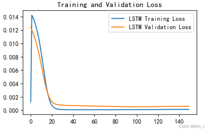
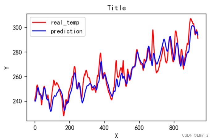
2. 调用模型进行预测
python
model.load_state_dict(best_model_wst)
model.to("cpu")
predicted_y_lstm = sc.inverse_transform(model(X_test).detach().numpy().reshape(-1,1))                    # 测试集输入模型进行预测
y_test_1 = sc.inverse_transform(y_test.reshape(-1,1))
y_test_one = [i[0] for i in y_test_1]
predicted_y_lstm_one = [i[0] for i in predicted_y_lstm]

plt.figure(figsize=(5, 3),dpi=120)
# 画出真实数据和预测数据的对比曲线
plt.plot(y_test_one[:2000], color='red', label='real_temp')
plt.plot(predicted_y_lstm_one[:2000], color='blue', label='prediction')

plt.title('Title')
plt.xlabel('X')
plt.ylabel('Y')
plt.legend()
plt.show()
3. R2值评估
python
from sklearn import metrics
"""
RMSE :均方根误差  ----->  对均方误差开方
R2   :决定系数,可以简单理解为反映模型拟合优度的重要的统计量
"""
RMSE_lstm  = metrics.mean_squared_error(predicted_y_lstm_one, y_test_1)**0.5
R2_lstm    = metrics.r2_score(predicted_y_lstm_one, y_test_1)

print('均方根误差: %.5f' % RMSE_lstm)
print('R2: %.5f' % R2_lstm)
输出:
python
均方根误差: 6.53662
R2: 0.85083
五、总结
在数据预测前,数据预处理极为关键,包含数据去重、去空值。在设置迭代次数时,可适量缩小迭代次数。