吴恩达老师机器学习-ex2

有借鉴网上的部分

第一题

导入库，读取数据并且展示前五行（基本操作）

复制代码

import numpy as np
import pandas as pd
import matplotlib.pyplot as plt
#读取数据
path = "./ex2data1.txt"
data = pd.read_csv(path,header=None,names=["exam1","exam2","accepted"])
print(data.head())

可视化数据

将数据集绘制成散点图，这里采用了子图绘制的方式，返回的fig和ax对象分别代表了整个图形和其中的一个子图。x，y分别为每个样本的exam1和exam2，通过accepted区分蓝色和红色。

复制代码

fig,ax=plt.subplots()
ax.scatter(data[data["accepted"]==0]["exam1"],data[data["accepted"]==0]["exam2"],c="r",marker="x")
ax.scatter(data[data["accepted"]==1]["exam1"],data[data["accepted"]==1]["exam2"],c="b",marker="o")
ax.set_xlabel('exam1')  
ax.set_ylabel('exam2')
plt.show()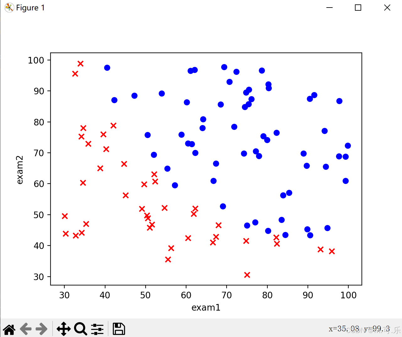

读取x，y

先添加一列为1，x为特征值，y为真实值

复制代码

data.insert(0,"x0",1)
cols = data.shape[1]
x = data.iloc[:,0:cols-1]
y = data.iloc[:,cols-1:cols]
x = x.values
y = y.values.reshape(len(y), 1)
theta = np.zeros((3,1))

构造损失函数

损失函数公式为

其中，

复制代码

def cost_func(x,y,theta):
    z = x@theta
    A = 1/(1+np.exp(-z))
    cost = -np.sum(y*np.log(A)+(1-y)*np.log(1-A))/len(x)
    return cost

构造梯度下降函数

复制代码

def gradient_descent(x,y,theta,alpha,times):
    m = len(x)
    for i in range(times):
        z = x@theta
        A = 1/(1+np.exp(-z))
        theta = theta - (alpha / m) * (x.T@(A-y))
        cost = cost_func(x,y,theta)
        pass
    return theta

初始化

复制代码

alpha = 0.004
times = 200000
theta = gradient_descent(x,y,theta,alpha,times)

决策界限

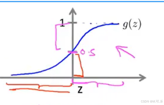
根据sigmoid函数（如图所示），当为边界线，也就是。

所以，并且为我们新添加的一列1，可以推出

所以

然后，绘制出图像，散点图和决策边界

复制代码

conf1 = -theta[0,0]/theta[2,0]
conf2 = -theta[1,0]/theta[2,0]
x = np.linspace(20, 100, 100)
y = conf1+conf2*x
fig,ax=plt.subplots()
ax.scatter(data[data["accepted"]==0]["exam1"],data[data["accepted"]==0]["exam2"],c="r",marker="x")
ax.scatter(data[data["accepted"]==1]["exam1"],data[data["accepted"]==1]["exam2"],c="b",marker="o")
ax.plot(x,y,c="g")
ax.set_xlabel('exam1') 
ax.set_ylabel('exam2')
plt.show()

第二题

导入库，读取数据并且展示前五行（基本操作）

复制代码

import numpy as np
import pandas as pd
import matplotlib.pyplot as plt

#读取数据
path = "./ex2data2.txt"
data = pd.read_csv(path,header = None,names = ["exam1","exam2","accepted"])
print(data.head())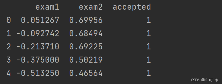

可视化数据

复制代码

fig,ax=plt.subplots()
ax.scatter(data[data["accepted"]==0]["exam1"],data[data["accepted"]==0]["exam2"],c="r",marker="x")
ax.scatter(data[data["accepted"]==1]["exam1"],data[data["accepted"]==1]["exam2"],c="b",marker="o")
ax.set_xlabel('exam1')
ax.set_ylabel('exam2')
plt.show()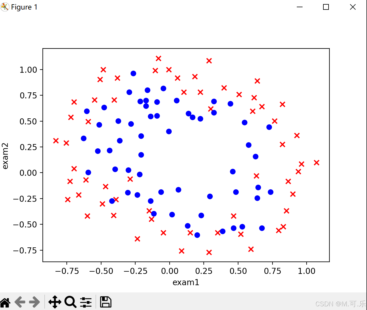

特征映射

通过上面绘制的散点图，我么可以看出来，该题目是线性不可分的，所以我们要增加项的次数，采用的是特征映射的方式

复制代码

def feature_mapping(x1,x2,times):
    data = {}
    for i in range(times+1):
        for j in range(i+1):
            data["F{}{}".format(i-j,j)] = np.power(x1,i-j)*np.power(x2,j)
    return pd.DataFrame(data)
x1 = data["exam1"]
x2 = data["exam2"]
data_finite = feature_mapping(x1,x2,6)

读取x，y

因为在特征映射时，可以根据公式看出第一列已经为0

复制代码

cols = data.shape[1]
x = data_finite.values
y = data.iloc[:,cols-1:cols]
y = y.values
theta = np.zeros((28,1))

构造代价函数

跟第一题不同的是，这里要加入正则化，为了防止过拟合现象

复制代码

def cost_func(x,y,theta,lamda):
    z = x@theta
    A = 1/(1+np.exp(-z))
    m = len(x)
    cost = np.sum(-y*np.log(A)-(1-y)*np.log(1-A))/m
    reg = np.sum(np.power(theta[1:],2))*(lamda/2*m)
    return cost+reg

构造梯度下降函数

复制代码

def gradient_descent(x, y, theta, alpha, iters, lamda):
    for i in range(iters):
        reg = theta[1:] * (lamda / len(x))
        reg = np.insert(reg, 0, values=0, axis=0)
        z = x @ theta
        A = 1 / (1 + np.exp(-z))
        # X.T:X的转置
        theta = theta - (x.T @ (A - y)) * alpha / len(x) - reg*alpha
        cost = cost_func(x, y, theta, lamda)
    return theta

初始化

复制代码

alpha = 0.001
times = 200000
lamda = 0.01
theta = gradient_descent(x,y,theta,alpha,times,lamda)

决策界限

这里我么需要画出决策界限（非线性）

首先，我们先调用meshgrid函数，得到网格中的坐标对应的x，y值。

复制代码

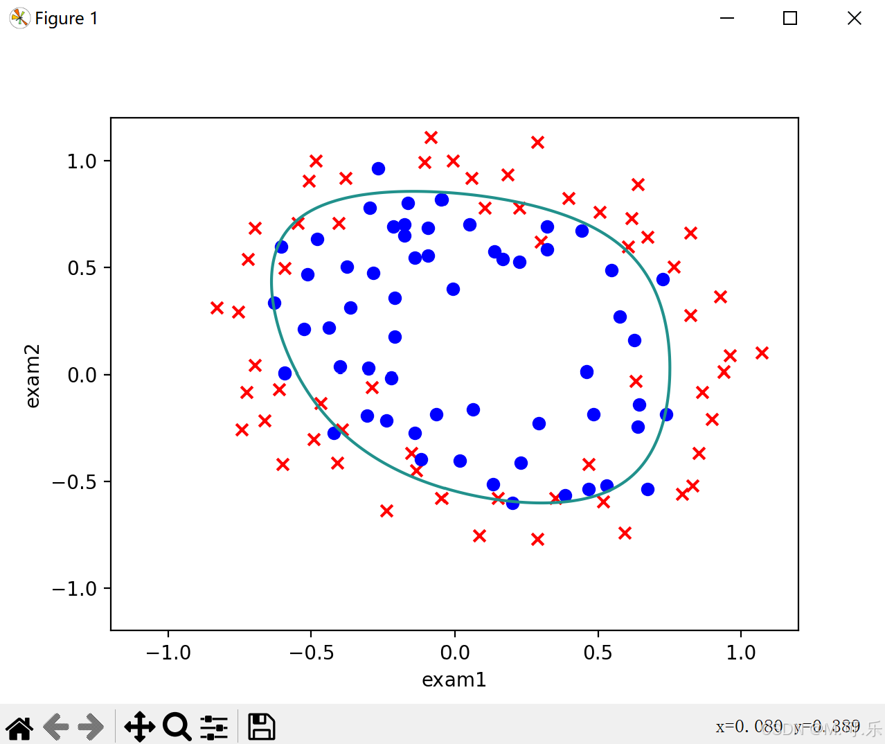
x = np.linspace(-1.2, 1.2, 200)
X,Y = np.meshgrid(x,x)
z = feature_mapping(X.ravel(), Y.ravel(), 6).values
Z = z @ theta
Z = Z.reshape(X.shape)
fig, ax = plt.subplots()
ax.scatter(data[data['accepted'] == 0]['exam1'], data[data['accepted'] == 0]['exam2'], c='r', marker='x')
ax.scatter(data[data['accepted'] == 1]['exam1'], data[data['accepted'] == 1]['exam2'], c='b', marker='o')
ax.set_xlabel('exam1')
ax.set_ylabel('exam2')
plt.contour(X, Y, Z, 0)
plt.show()