机器学习-决策树

python 复制代码

import numpy as np
import matplotlib.pyplot as plt
from sklearn import datasets

iris = datasets.load_iris()
X = iris.data[:,2:]
y = iris.target
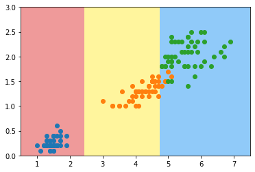
plt.scatter(X[y==0,0], X[y==0,1])
plt.scatter(X[y==1,0], X[y==1,1])
plt.scatter(X[y==2,0], X[y==2,1])
plt.show()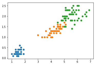

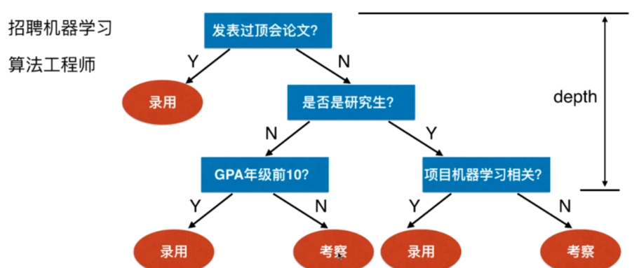
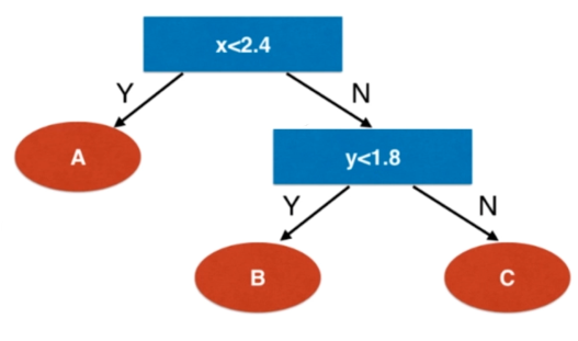
决策树

python 复制代码

from sklearn.tree import DecisionTreeClassifier

dt_clf = DecisionTreeClassifier(max_depth=2, criterion="entropy", random_state=42)
dt_clf.fit(X, y)

python 复制代码

def plot_decision_boundary(model, axis):
    
    x0, x1 = np.meshgrid(
        np.linspace(axis[0], axis[1], int((axis[1]-axis[0])*100)).reshape(-1, 1),
        np.linspace(axis[2], axis[3], int((axis[3]-axis[2])*100)).reshape(-1, 1),
    )
    X_new = np.c_[x0.ravel(), x1.ravel()]

    y_predict = model.predict(X_new)
    zz = y_predict.reshape(x0.shape)

    from matplotlib.colors import ListedColormap
    custom_cmap = ListedColormap(['#EF9A9A','#FFF59D','#90CAF9'])
    
    plt.contourf(x0, x1, zz, cmap=custom_cmap)

python 复制代码

plot_decision_boundary(dt_clf, axis=[0.5, 7.5, 0, 3])
plt.scatter(X[y==0,0], X[y==0,1])
plt.scatter(X[y==1,0], X[y==1,1])
plt.scatter(X[y==2,0], X[y==2,1])
plt.show()

非参数学习算法

可以解决分类问题

天然可以解决多分类问题

也可以解决回归问题

非常好的可解释性

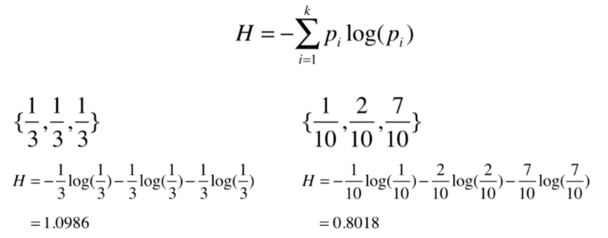
信息熵

熵在信息论中代表随机变量不确定度的度量

熵越大，数据的不确定性越高

熵越小，数据的不确定性越低

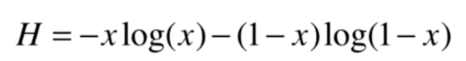
可视化

python 复制代码

import numpy as np
import matplotlib.pyplot as plt
def entropy(p):
    return -p * np.log(p) - (1-p) * np.log(1-p)
x = np.linspace(0.01, 0.99, 200)
plt.plot(x, entropy(x))
plt.show()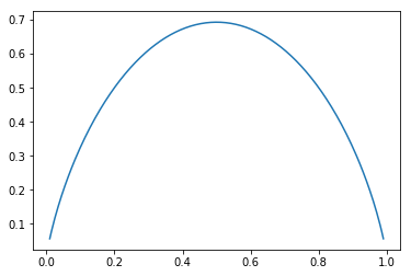

使用信息熵寻找最优划分

python 复制代码

import numpy as np
import matplotlib.pyplot as plt
from sklearn import datasets

iris = datasets.load_iris()
X = iris.data[:,2:]
y = iris.target
from sklearn.tree import DecisionTreeClassifier

dt_clf = DecisionTreeClassifier(max_depth=2, criterion="entropy", random_state=42)
dt_clf.fit(X, y)

python 复制代码

def plot_decision_boundary(model, axis):
    
    x0, x1 = np.meshgrid(
        np.linspace(axis[0], axis[1], int((axis[1]-axis[0])*100)).reshape(-1, 1),
        np.linspace(axis[2], axis[3], int((axis[3]-axis[2])*100)).reshape(-1, 1),
    )
    X_new = np.c_[x0.ravel(), x1.ravel()]

    y_predict = model.predict(X_new)
    zz = y_predict.reshape(x0.shape)

    from matplotlib.colors import ListedColormap
    custom_cmap = ListedColormap(['#EF9A9A','#FFF59D','#90CAF9'])
    
    plt.contourf(x0, x1, zz, cmap=custom_cmap)

python 复制代码

plot_decision_boundary(dt_clf, axis=[0.5, 7.5, 0, 3])
plt.scatter(X[y==0,0], X[y==0,1])
plt.scatter(X[y==1,0], X[y==1,1])
plt.scatter(X[y==2,0], X[y==2,1])
plt.show()

模拟使用信息熵进行划分

python 复制代码

def split(X, y, d, value):
    index_a = (X[:,d] <= value)
    index_b = (X[:,d] > value)
    return X[index_a], X[index_b], y[index_a], y[index_b]

python 复制代码

from collections import Counter
from math import log

def entropy(y):
    counter = Counter(y)
    res = 0.0
    for num in counter.values():
        p = num / len(y)
        res += -p * log(p)
    return res

def try_split(X, y):
    
    best_entropy = float('inf')
    best_d, best_v = -1, -1
    for d in range(X.shape[1]):
        sorted_index = np.argsort(X[:,d])
        for i in range(1, len(X)):
            if X[sorted_index[i], d] != X[sorted_index[i-1], d]:
                v = (X[sorted_index[i], d] + X[sorted_index[i-1], d])/2
                X_l, X_r, y_l, y_r = split(X, y, d, v)
                p_l, p_r = len(X_l) / len(X), len(X_r) / len(X)
                e = p_l * entropy(y_l) + p_r * entropy(y_r)
                if e < best_entropy:
                    best_entropy, best_d, best_v = e, d, v
                
    return best_entropy, best_d, best_v

python 复制代码

best_entropy, best_d, best_v = try_split(X, y)
print("best_entropy =", best_entropy)
print("best_d =", best_d)
print("best_v =", best_v)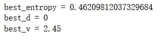

python 复制代码

X1_l, X1_r, y1_l, y1_r = split(X, y, best_d, best_v)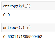

python 复制代码

best_entropy2, best_d2, best_v2 = try_split(X1_r, y1_r)
print("best_entropy =", best_entropy2)
print("best_d =", best_d2)
print("best_v =", best_v2)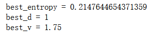

python 复制代码

X2_l, X2_r, y2_l, y2_r = split(X1_r, y1_r, best_d2, best_v2)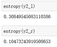

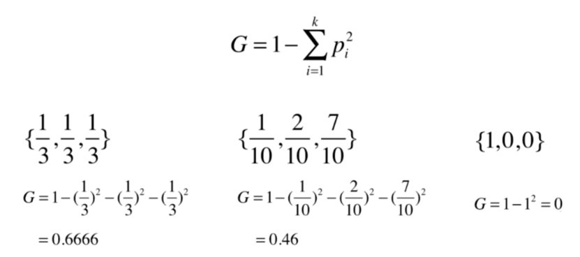
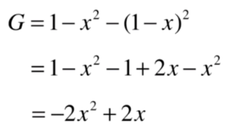
基尼系数

python 复制代码

import numpy as np
import matplotlib.pyplot as plt

python 复制代码

from sklearn import datasets

iris = datasets.load_iris()
X = iris.data[:,2:]
y = iris.target

python 复制代码

from sklearn.tree import DecisionTreeClassifier

dt_clf = DecisionTreeClassifier(max_depth=2, criterion="gini", random_state=42)
dt_clf.fit(X, y)

python 复制代码

def plot_decision_boundary(model, axis):
    
    x0, x1 = np.meshgrid(
        np.linspace(axis[0], axis[1], int((axis[1]-axis[0])*200)).reshape(-1, 1),
        np.linspace(axis[2], axis[3], int((axis[3]-axis[2])*200)).reshape(-1, 1),
    )
    X_new = np.c_[x0.ravel(), x1.ravel()]

    y_predict = model.predict(X_new)
    zz = y_predict.reshape(x0.shape)

    from matplotlib.colors import ListedColormap
    custom_cmap = ListedColormap(['#EF9A9A','#FFF59D','#90CAF9'])
    
    plt.contourf(x0, x1, zz, cmap=custom_cmap)

python 复制代码

plot_decision_boundary(dt_clf, axis=[0.5, 7.5, 0, 3])
plt.scatter(X[y==0,0], X[y==0,1])
plt.scatter(X[y==1,0], X[y==1,1])
plt.scatter(X[y==2,0], X[y==2,1])
plt.show()

模拟使用基尼系数划分

python 复制代码

from collections import Counter
from math import log

def split(X, y, d, value):
    index_a = (X[:,d] <= value)
    index_b = (X[:,d] > value)
    return X[index_a], X[index_b], y[index_a], y[index_b]

def gini(y):
    counter = Counter(y)
    res = 1.0
    for num in counter.values():
        p = num / len(y)
        res -= p**2
    return res

def try_split(X, y):
    
    best_g = float('inf')
    best_d, best_v = -1, -1
    for d in range(X.shape[1]):
        sorted_index = np.argsort(X[:,d])
        for i in range(1, len(X)):
            if X[sorted_index[i], d] != X[sorted_index[i-1], d]:
                v = (X[sorted_index[i], d] + X[sorted_index[i-1], d])/2
                X_l, X_r, y_l, y_r = split(X, y, d, v)
                p_l, p_r = len(X_l) / len(X), len(X_r) / len(X)
                g = p_l * gini(y_l) + p_r * gini(y_r)
                if g < best_g:
                    best_g, best_d, best_v = g, d, v
                
    return best_g, best_d, best_v

python 复制代码

best_g, best_d, best_v = try_split(X, y)
print("best_g =", best_g)
print("best_d =", best_d)
print("best_v =", best_v)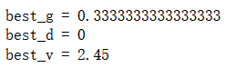

python 复制代码

X1_l, X1_r, y1_l, y1_r = split(X, y, best_d, best_v)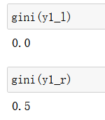

python 复制代码

best_g2, best_d2, best_v2 = try_split(X1_r, y1_r)
print("best_g =", best_g2)
print("best_d =", best_d2)
print("best_v =", best_v2)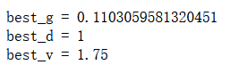

python 复制代码

X2_l, X2_r, y2_l, y2_r = split(X1_r, y1_r, best_d2, best_v2)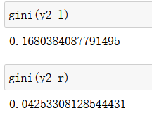

信息熵 vs 基尼系数

熵信息的计算比基尼系数稍慢

scikit-learn中默认为基尼系数

大多数时候二者没有特别的效果优劣

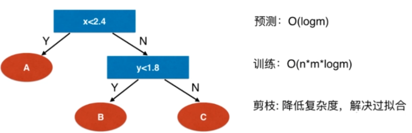
CART与决策树中的超参数

CART

Classification And Regression Tree

根据某一个维度d和某一个阈值v进行二分

scikit-learn的决策树实现:CART

ID3, C4.5, C5.0

复杂度

python 复制代码

import numpy as np
import matplotlib.pyplot as plt

python 复制代码

from sklearn import datasets

X, y = datasets.make_moons(noise=0.25, random_state=666)

python 复制代码

plt.scatter(X[y==0,0], X[y==0,1])
plt.scatter(X[y==1,0], X[y==1,1])
plt.show()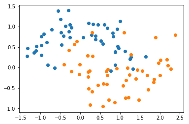

python 复制代码

from sklearn.tree import DecisionTreeClassifier

dt_clf = DecisionTreeClassifier()
dt_clf.fit(X, y)

python 复制代码

def plot_decision_boundary(model, axis):
    
    x0, x1 = np.meshgrid(
        np.linspace(axis[0], axis[1], int((axis[1]-axis[0])*100)).reshape(-1, 1),
        np.linspace(axis[2], axis[3], int((axis[3]-axis[2])*100)).reshape(-1, 1),
    )
    X_new = np.c_[x0.ravel(), x1.ravel()]

    y_predict = model.predict(X_new)
    zz = y_predict.reshape(x0.shape)

    from matplotlib.colors import ListedColormap
    custom_cmap = ListedColormap(['#EF9A9A','#FFF59D','#90CAF9'])
    
    plt.contourf(x0, x1, zz, linewidth=5, cmap=custom_cmap)

python 复制代码

plot_decision_boundary(dt_clf, axis=[-1.5, 2.5, -1.0, 1.5])
plt.scatter(X[y==0,0], X[y==0,1])
plt.scatter(X[y==1,0], X[y==1,1])
plt.show()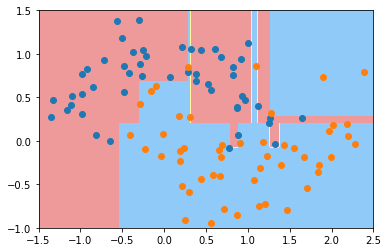

python 复制代码

dt_clf2 = DecisionTreeClassifier(max_depth=2)
dt_clf2.fit(X, y)

plot_decision_boundary(dt_clf2, axis=[-1.5, 2.5, -1.0, 1.5])
plt.scatter(X[y==0,0], X[y==0,1])
plt.scatter(X[y==1,0], X[y==1,1])
plt.show()

python 复制代码

dt_clf3 = DecisionTreeClassifier(min_samples_split=10)
dt_clf3.fit(X, y)

plot_decision_boundary(dt_clf3, axis=[-1.5, 2.5, -1.0, 1.5])
plt.scatter(X[y==0,0], X[y==0,1])
plt.scatter(X[y==1,0], X[y==1,1])
plt.show()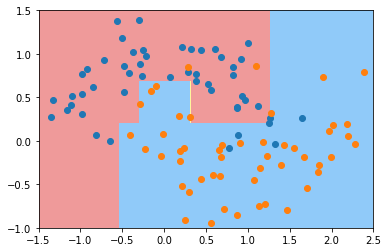

python 复制代码

dt_clf4 = DecisionTreeClassifier(min_samples_leaf=6)
dt_clf4.fit(X, y)

plot_decision_boundary(dt_clf4, axis=[-1.5, 2.5, -1.0, 1.5])
plt.scatter(X[y==0,0], X[y==0,1])
plt.scatter(X[y==1,0], X[y==1,1])
plt.show()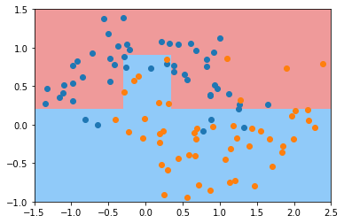

python 复制代码

dt_clf5 = DecisionTreeClassifier(max_leaf_nodes=4)
dt_clf5.fit(X, y)

plot_decision_boundary(dt_clf5, axis=[-1.5, 2.5, -1.0, 1.5])
plt.scatter(X[y==0,0], X[y==0,1])
plt.scatter(X[y==1,0], X[y==1,1])
plt.show()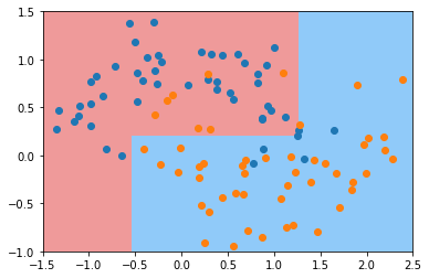

min_samples_split

min_samples leaf

min_weight fraction leaf

max depth

max leaf nodesmin features

http://scikit-learn.org/stable/modules/generated/sklearn.tree.DecisionTreeClassifier.html#sklearn.tree.DecisionTreeClassifier

决策树解决回归问题

python 复制代码

import numpy as np
import matplotlib.pyplot as plt

python 复制代码

from sklearn import datasets

boston = datasets.load_boston()
X = boston.data
y = boston.target

python 复制代码

from sklearn.model_selection import train_test_split

X_train, X_test, y_train, y_test = train_test_split(X, y, random_state=666)

python 复制代码

from sklearn.tree import DecisionTreeRegressor

dt_reg = DecisionTreeRegressor()
dt_reg.fit(X_train, y_train)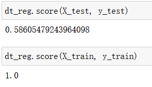

模型复杂度曲线

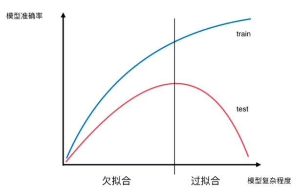
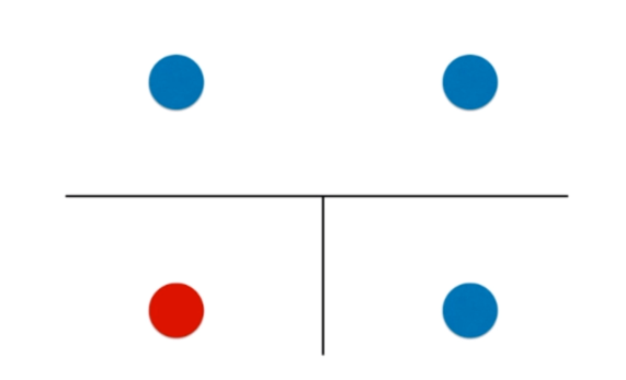
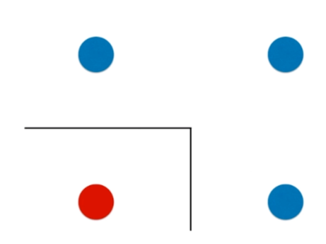
决策树的局限性

python 复制代码

import numpy as np
import matplotlib.pyplot as plt

python 复制代码

from sklearn import datasets

iris = datasets.load_iris()
X = iris.data[:,2:]
y = iris.target

python 复制代码

from sklearn.tree import DecisionTreeClassifier

tree_clf = DecisionTreeClassifier(max_depth=2, criterion="entropy", random_state=42)
tree_clf.fit(X, y)

python 复制代码

def plot_decision_boundary(model, axis):
    
    x0, x1 = np.meshgrid(
        np.linspace(axis[0], axis[1], int((axis[1]-axis[0])*200)).reshape(-1, 1),
        np.linspace(axis[2], axis[3], int((axis[3]-axis[2])*200)).reshape(-1, 1),
    )
    X_new = np.c_[x0.ravel(), x1.ravel()]

    y_predict = model.predict(X_new)
    zz = y_predict.reshape(x0.shape)

    from matplotlib.colors import ListedColormap
    custom_cmap = ListedColormap(['#EF9A9A','#FFF59D','#90CAF9'])
    
    plt.contourf(x0, x1, zz, linewidth=5, cmap=custom_cmap)

python 复制代码

plot_decision_boundary(tree_clf, axis=[0.5, 7.5, 0, 3])
plt.scatter(X[y==0,0], X[y==0,1])
plt.scatter(X[y==1,0], X[y==1,1])
plt.scatter(X[y==2,0], X[y==2,1])
plt.show()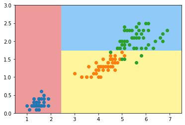

python 复制代码

X_new = np.delete(X, 106, axis=0)
y_new = np.delete(y, 106)

python 复制代码

tree_clf2 = DecisionTreeClassifier(max_depth=2, criterion="entropy", random_state=42)
tree_clf2.fit(X_new, y_new)

python 复制代码

plot_decision_boundary(tree_clf2, axis=[0.5, 7.5, 0, 3])
plt.scatter(X_new[y_new==0,0], X_new[y_new==0,1])
plt.scatter(X_new[y_new==1,0], X_new[y_new==1,1])
plt.scatter(X_new[y_new==2,0], X_new[y_new==2,1])
plt.show()