深度学习作业十 BPTT

目录

[习题6-1P 推导RNN反向传播算法BPTT.](#习题6-1P 推导RNN反向传播算法BPTT.)

[习题6-2 推导公式(6.40)和公式(6.41)中的梯度．](#习题6-2 推导公式(6.40)和公式(6.41)中的梯度．)

[习题6-3 当使用公式(6.50)作为循环神经网络的状态更新公式时， 分析其可能存在梯度爆炸的原因并给出解决方法．](#习题6-3 当使用公式(6.50)作为循环神经网络的状态更新公式时， 分析其可能存在梯度爆炸的原因并给出解决方法．)

[习题6-2P 设计简单RNN模型，分别用Numpy、Pytorch实现反向传播算子，并代入数值测试.](#习题6-2P 设计简单RNN模型，分别用Numpy、Pytorch实现反向传播算子，并代入数值测试.)

（1）RNNCell前向传播

（2）RNNcell反向传播

（3）RNN前向传播

（4）RNN反向传播

（5）分别用numpy和torch实现前向和反向传播

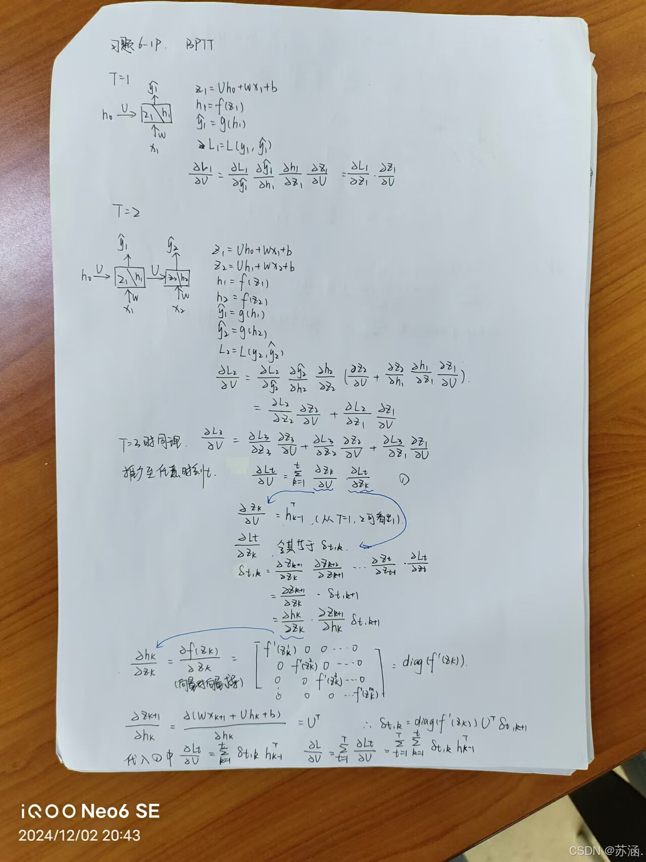
习题6-1P 推导RNN反向传播算法BPTT.

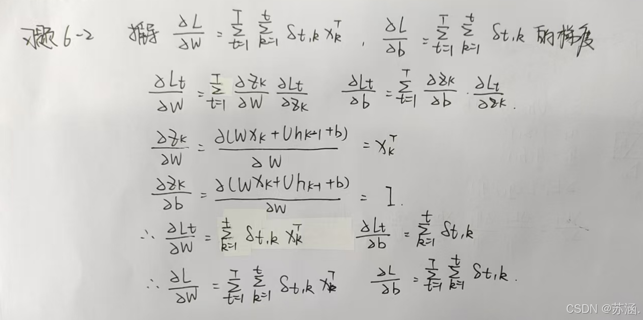
习题6-2 推导公式(6.40)和公式(6.41)中的梯度．

习题6-3 当使用公式(6.50)作为循环神经网络的状态更新公式时， 分析其可能存在梯度爆炸的原因并给出解决方法．

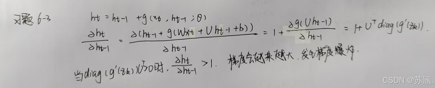
解决方法：

可以通过引入门控机制来进一步改进模型，主要有：长短期记忆网络（LSTM）和门控循环单元网络（GRU）。

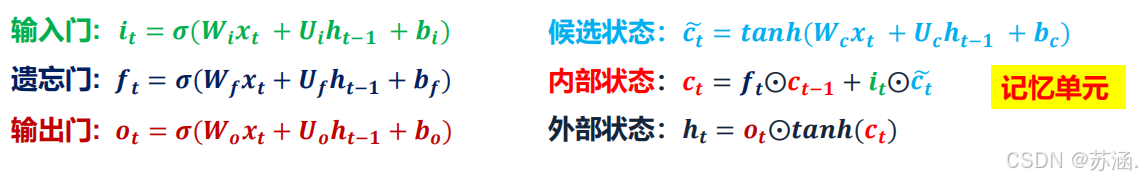
LSTM：

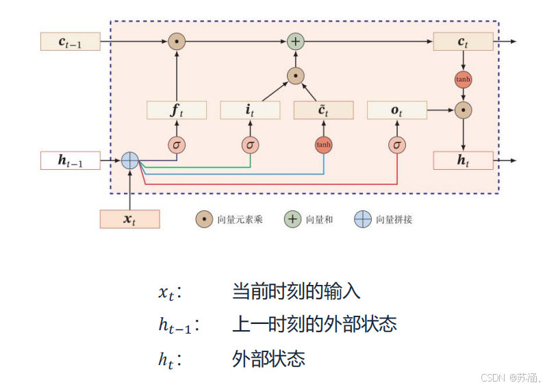
LSTM 通过引入多个门控机制（输入门、遗忘门和输出门）以及一个独立的细胞状态（Cell State），来实现对信息的选择性记忆和遗忘，从而捕捉长序列的依赖关系。

关键组件：

优点

• 能够捕捉长期依赖关系。
• 对梯度消失问题有较好的抑制效果。

缺点

• 结构复杂，参数较多，训练时间长。
• 在某些任务中可能存在过拟合问题。

---

GRU：

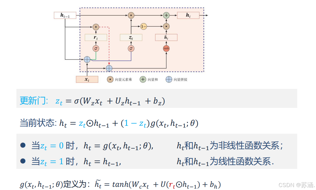
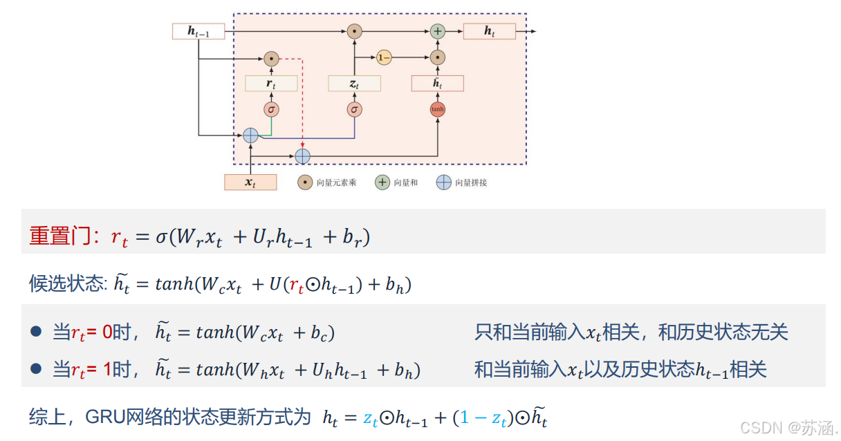
GRU 是 LSTM 的简化版本，融合了遗忘门和输入门，减少了网络的复杂性，同时保持了对长序列依赖关系的建模能力。

优点

• 参数比 LSTM 更少，计算效率更高。
• 能在某些任务中达到与 LSTM 类似的性能。

缺点

• 不具备 LSTM 的完全灵活性，在极长序列任务中可能表现略逊色。

习题6-2P 设计简单RNN模型，分别用Numpy、Pytorch实现反向传播算子，并代入数值测试.

（1）RNNCell前向传播

代码如下：

# ======RNNcell前向传播==================================================================
def rnn_cell_forward(xt, a_prev, parameters):
    # Retrieve parameters from "parameters"
    Wax = parameters["Wax"]
    Waa = parameters["Waa"]
    Wya = parameters["Wya"]
    ba = parameters["ba"]
    by = parameters["by"]

    ### START CODE HERE ### (≈2 lines)
    # compute next activation state using the formula given above
    a_next = np.tanh(np.dot(Wax, xt) + np.dot(Waa, a_prev) + ba)
    # compute output of the current cell using the formula given above
    yt_pred = F.softmax(torch.from_numpy(np.dot(Wya, a_next) + by), dim=0)
    ### END CODE HERE ###

    # store values you need for backward propagation in cache
    cache = (a_next, a_prev, xt, parameters)

    return a_next, yt_pred, cache


np.random.seed(1)
xt = np.random.randn(3, 10)
a_prev = np.random.randn(5, 10)
Waa = np.random.randn(5, 5)
Wax = np.random.randn(5, 3)
Wya = np.random.randn(2, 5)
ba = np.random.randn(5, 1)
by = np.random.randn(2, 1)
parameters = {"Waa": Waa, "Wax": Wax, "Wya": Wya, "ba": ba, "by": by}

a_next, yt_pred, cache = rnn_cell_forward(xt, a_prev, parameters)
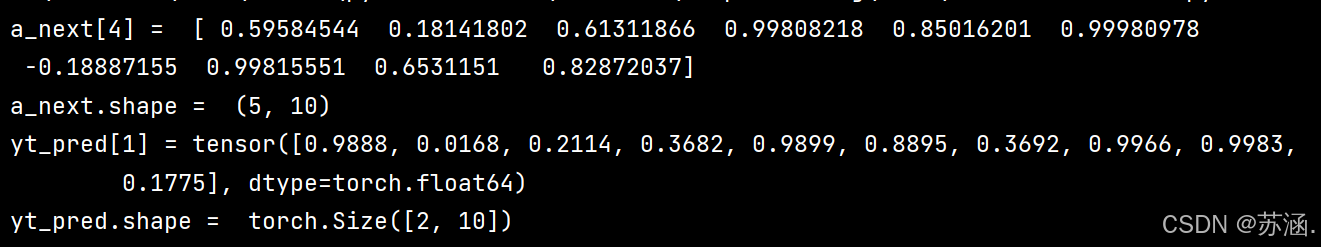
print("a_next[4] = ", a_next[4])
print("a_next.shape = ", a_next.shape)
print("yt_pred[1] =", yt_pred[1])
print("yt_pred.shape = ", yt_pred.shape)
print("===================================================================")

运行结果：

（2）RNNcell反向传播

代码如下：

# ======RNNcell反向传播========================================================
def rnn_cell_backward(da_next, cache):
    # Retrieve values from cache
    (a_next, a_prev, xt, parameters) = cache

    # Retrieve values from parameters
    Wax = parameters["Wax"]
    Waa = parameters["Waa"]
    Wya = parameters["Wya"]
    ba = parameters["ba"]
    by = parameters["by"]

    ### START CODE HERE ###
    # compute the gradient of tanh with respect to a_next (≈1 line)
    dtanh = (1 - a_next * a_next) * da_next  # 注意这里是 element_wise ,即 * da_next，dtanh 可以只看做一个中间结果的表示方式

    # compute the gradient of the loss with respect to Wax (≈2 lines)
    dxt = np.dot(Wax.T, dtanh)
    dWax = np.dot(dtanh, xt.T)
    # 根据公式1、2， dxt =  da_next .(  Wax.T  . (1- tanh(a_next)**2) ) = da_next .(  Wax.T  . dtanh * (1/d_a_next) )= Wax.T  . dtanh
    # 根据公式1、3， dWax =  da_next .( (1- tanh(a_next)**2) . xt.T) = da_next .(  dtanh * (1/d_a_next) . xt.T )=  dtanh . xt.T
    # 上面的 . 表示 np.dot

    # compute the gradient with respect to Waa (≈2 lines)
    da_prev = np.dot(Waa.T, dtanh)
    dWaa = np.dot(dtanh, a_prev.T)

    # compute the gradient with respect to b (≈1 line)
    dba = np.sum(dtanh, keepdims=True, axis=-1)  # axis=0 列方向上操作 axis=1 行方向上操作  keepdims=True 矩阵的二维特性

    ### END CODE HERE ###

    # Store the gradients in a python dictionary
    gradients = {"dxt": dxt, "da_prev": da_prev, "dWax": dWax, "dWaa": dWaa, "dba": dba}

    return gradients


np.random.seed(1)
xt = np.random.randn(3, 10)
a_prev = np.random.randn(5, 10)
Wax = np.random.randn(5, 3)
Waa = np.random.randn(5, 5)
Wya = np.random.randn(2, 5)
b = np.random.randn(5, 1)
by = np.random.randn(2, 1)
parameters = {"Wax": Wax, "Waa": Waa, "Wya": Wya, "ba": ba, "by": by}

a_next, yt, cache = rnn_cell_forward(xt, a_prev, parameters)

da_next = np.random.randn(5, 10)
gradients = rnn_cell_backward(da_next, cache)
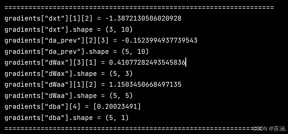
print("gradients[\"dxt\"][1][2] =", gradients["dxt"][1][2])
print("gradients[\"dxt\"].shape =", gradients["dxt"].shape)
print("gradients[\"da_prev\"][2][3] =", gradients["da_prev"][2][3])
print("gradients[\"da_prev\"].shape =", gradients["da_prev"].shape)
print("gradients[\"dWax\"][3][1] =", gradients["dWax"][3][1])
print("gradients[\"dWax\"].shape =", gradients["dWax"].shape)
print("gradients[\"dWaa\"][1][2] =", gradients["dWaa"][1][2])
print("gradients[\"dWaa\"].shape =", gradients["dWaa"].shape)
print("gradients[\"dba\"][4] =", gradients["dba"][4])
print("gradients[\"dba\"].shape =", gradients["dba"].shape)
gradients["dxt"][1][2] = -0.4605641030588796
gradients["dxt"].shape = (3, 10)
gradients["da_prev"][2][3] = 0.08429686538067724
gradients["da_prev"].shape = (5, 10)
gradients["dWax"][3][1] = 0.39308187392193034
gradients["dWax"].shape = (5, 3)
gradients["dWaa"][1][2] = -0.28483955786960663
gradients["dWaa"].shape = (5, 5)
gradients["dba"][4] = [0.80517166]
gradients["dba"].shape = (5, 1)
print("================================================================")

运行结果：

（3）RNN前向传播

代码如下：

# ====RNN前向传播==============================================================
def rnn_forward(x, a0, parameters):
    # Initialize "caches" which will contain the list of all caches
    caches = []

    # Retrieve dimensions from shapes of x and Wy
    n_x, m, T_x = x.shape
    n_y, n_a = parameters["Wya"].shape

    ### START CODE HERE ###

    # initialize "a" and "y" with zeros (≈2 lines)
    a = np.zeros((n_a, m, T_x))
    y_pred = np.zeros((n_y, m, T_x))

    # Initialize a_next (≈1 line)
    a_next = a0

    # loop over all time-steps
    for t in range(T_x):
        # Update next hidden state, compute the prediction, get the cache (≈1 line)
        a_next, yt_pred, cache = rnn_cell_forward(x[:, :, t], a_next, parameters)
        # Save the value of the new "next" hidden state in a (≈1 line)
        a[:, :, t] = a_next
        # Save the value of the prediction in y (≈1 line)
        y_pred[:, :, t] = yt_pred
        # Append "cache" to "caches" (≈1 line)
        caches.append(cache)

    ### END CODE HERE ###

    # store values needed for backward propagation in cache
    caches = (caches, x)

    return a, y_pred, caches


np.random.seed(1)
x = np.random.randn(3, 10, 4)
a0 = np.random.randn(5, 10)
Waa = np.random.randn(5, 5)
Wax = np.random.randn(5, 3)
Wya = np.random.randn(2, 5)
ba = np.random.randn(5, 1)
by = np.random.randn(2, 1)
parameters = {"Waa": Waa, "Wax": Wax, "Wya": Wya, "ba": ba, "by": by}

a, y_pred, caches = rnn_forward(x, a0, parameters)
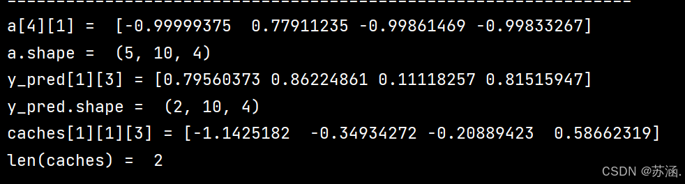
print("a[4][1] = ", a[4][1])
print("a.shape = ", a.shape)
print("y_pred[1][3] =", y_pred[1][3])
print("y_pred.shape = ", y_pred.shape)
print("caches[1][1][3] =", caches[1][1][3])
print("len(caches) = ", len(caches))
print("=============================================================")

运行结果：

（4）RNN反向传播

代码如下：

# =====RNN反向传播=================================================================
def rnn_backward(da, caches):
    ### START CODE HERE ###
    # Retrieve values from the first cache (t=1) of caches (≈2 lines)
    (caches, x) = caches
    (a1, a0, x1, parameters) = caches[0]  # t=1 时的值

    # Retrieve dimensions from da's and x1's shapes (≈2 lines)
    n_a, m, T_x = da.shape
    n_x, m = x1.shape

    # initialize the gradients with the right sizes (≈6 lines)
    dx = np.zeros((n_x, m, T_x))
    dWax = np.zeros((n_a, n_x))
    dWaa = np.zeros((n_a, n_a))
    dba = np.zeros((n_a, 1))
    da0 = np.zeros((n_a, m))
    da_prevt = np.zeros((n_a, m))

    # Loop through all the time steps
    for t in reversed(range(T_x)):
        # Compute gradients at time step t. Choose wisely the "da_next" and the "cache" to use in the backward propagation step. (≈1 line)
        gradients = rnn_cell_backward(da[:, :, t] + da_prevt, caches[t])  # da[:,:,t] + da_prevt ，每一个时间步后更新梯度
        # Retrieve derivatives from gradients (≈ 1 line)
        dxt, da_prevt, dWaxt, dWaat, dbat = gradients["dxt"], gradients["da_prev"], gradients["dWax"], gradients[
            "dWaa"], gradients["dba"]
        # Increment global derivatives w.r.t parameters by adding their derivative at time-step t (≈4 lines)
        dx[:, :, t] = dxt
        dWax += dWaxt
        dWaa += dWaat
        dba += dbat

    # Set da0 to the gradient of a which has been backpropagated through all time-steps (≈1 line)
    da0 = da_prevt
    ### END CODE HERE ###

    # Store the gradients in a python dictionary
    gradients = {"dx": dx, "da0": da0, "dWax": dWax, "dWaa": dWaa, "dba": dba}

    return gradients


np.random.seed(1)
x = np.random.randn(3, 10, 4)
a0 = np.random.randn(5, 10)
Wax = np.random.randn(5, 3)
Waa = np.random.randn(5, 5)
Wya = np.random.randn(2, 5)
ba = np.random.randn(5, 1)
by = np.random.randn(2, 1)
parameters = {"Wax": Wax, "Waa": Waa, "Wya": Wya, "ba": ba, "by": by}
a, y, caches = rnn_forward(x, a0, parameters)
da = np.random.randn(5, 10, 4)
gradients = rnn_backward(da, caches)

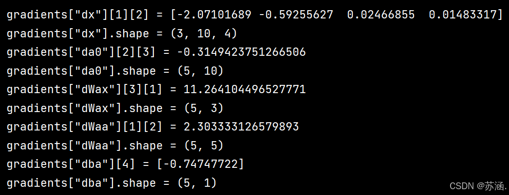
print("gradients[\"dx\"][1][2] =", gradients["dx"][1][2])
print("gradients[\"dx\"].shape =", gradients["dx"].shape)
print("gradients[\"da0\"][2][3] =", gradients["da0"][2][3])
print("gradients[\"da0\"].shape =", gradients["da0"].shape)
print("gradients[\"dWax\"][3][1] =", gradients["dWax"][3][1])
print("gradients[\"dWax\"].shape =", gradients["dWax"].shape)
print("gradients[\"dWaa\"][1][2] =", gradients["dWaa"][1][2])
print("gradients[\"dWaa\"].shape =", gradients["dWaa"].shape)
print("gradients[\"dba\"][4] =", gradients["dba"][4])
print("gradients[\"dba\"].shape =", gradients["dba"].shape)
print("===========================================================")

运行结果：

（5）分别用numpy和torch实现前向和反向传播

代码如下：

# =====分别用numpy和torch实现前向和反向传播===================================================
import torch
import numpy as np


class RNNCell:
    def __init__(self, weight_ih, weight_hh,
                 bias_ih, bias_hh):
        self.weight_ih = weight_ih
        self.weight_hh = weight_hh
        self.bias_ih = bias_ih
        self.bias_hh = bias_hh

        self.x_stack = []
        self.dx_list = []
        self.dw_ih_stack = []
        self.dw_hh_stack = []
        self.db_ih_stack = []
        self.db_hh_stack = []

        self.prev_hidden_stack = []
        self.next_hidden_stack = []

        # temporary cache
        self.prev_dh = None

    def __call__(self, x, prev_hidden):
        self.x_stack.append(x)

        next_h = np.tanh(
            np.dot(x, self.weight_ih.T)
            + np.dot(prev_hidden, self.weight_hh.T)
            + self.bias_ih + self.bias_hh)

        self.prev_hidden_stack.append(prev_hidden)
        self.next_hidden_stack.append(next_h)
        # clean cache
        self.prev_dh = np.zeros(next_h.shape)
        return next_h

    def backward(self, dh):
        x = self.x_stack.pop()
        prev_hidden = self.prev_hidden_stack.pop()
        next_hidden = self.next_hidden_stack.pop()

        d_tanh = (dh + self.prev_dh) * (1 - next_hidden ** 2)
        self.prev_dh = np.dot(d_tanh, self.weight_hh)

        dx = np.dot(d_tanh, self.weight_ih)
        self.dx_list.insert(0, dx)

        dw_ih = np.dot(d_tanh.T, x)
        self.dw_ih_stack.append(dw_ih)

        dw_hh = np.dot(d_tanh.T, prev_hidden)
        self.dw_hh_stack.append(dw_hh)

        self.db_ih_stack.append(d_tanh)
        self.db_hh_stack.append(d_tanh)

        return self.dx_list


if __name__ == '__main__':
    np.random.seed(123)
    torch.random.manual_seed(123)
    np.set_printoptions(precision=6, suppress=True)

    rnn_PyTorch = torch.nn.RNN(4, 5).double()
    rnn_numpy = RNNCell(rnn_PyTorch.all_weights[0][0].data.numpy(),
                        rnn_PyTorch.all_weights[0][1].data.numpy(),
                        rnn_PyTorch.all_weights[0][2].data.numpy(),
                        rnn_PyTorch.all_weights[0][3].data.numpy())

    nums = 3
    x3_numpy = np.random.random((nums, 3, 4))
    x3_tensor = torch.tensor(x3_numpy, requires_grad=True)

    h3_numpy = np.random.random((1, 3, 5))
    h3_tensor = torch.tensor(h3_numpy, requires_grad=True)

    dh_numpy = np.random.random((nums, 3, 5))
    dh_tensor = torch.tensor(dh_numpy, requires_grad=True)

    h3_tensor = rnn_PyTorch(x3_tensor, h3_tensor)
    h_numpy_list = []

    h_numpy = h3_numpy[0]
    for i in range(nums):
        h_numpy = rnn_numpy(x3_numpy[i], h_numpy)
        h_numpy_list.append(h_numpy)

    h3_tensor[0].backward(dh_tensor)
    for i in reversed(range(nums)):
        rnn_numpy.backward(dh_numpy[i])

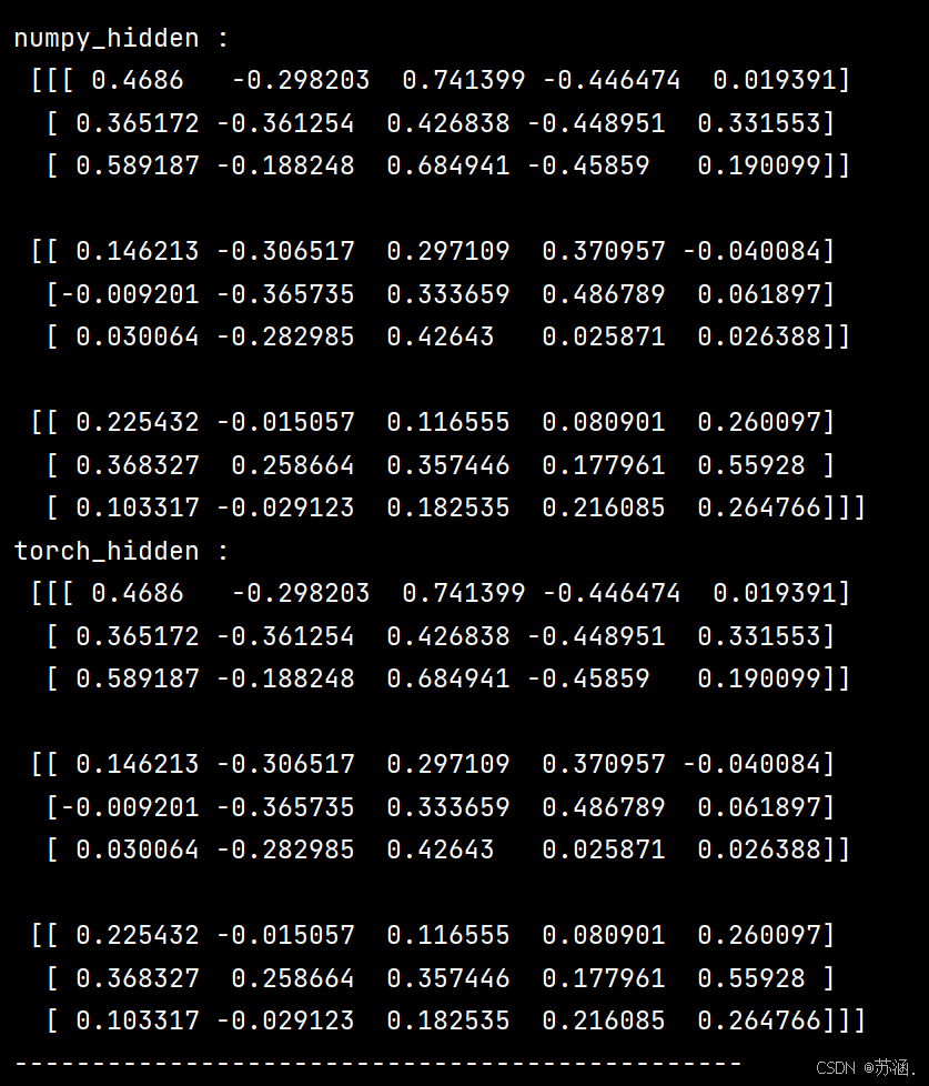
    print("numpy_hidden :\n", np.array(h_numpy_list))
    print("torch_hidden :\n", h3_tensor[0].data.numpy())
    print("-----------------------------------------------")

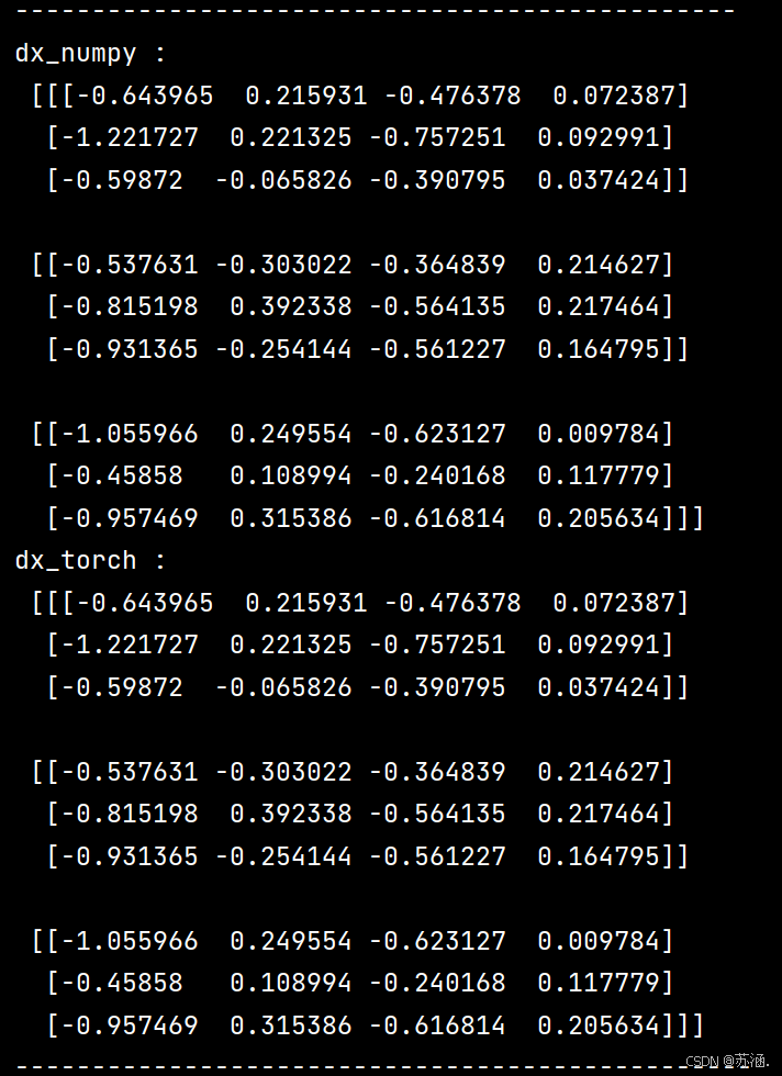
    print("dx_numpy :\n", np.array(rnn_numpy.dx_list))
    print("dx_torch :\n", x3_tensor.grad.data.numpy())
    print("------------------------------------------------")

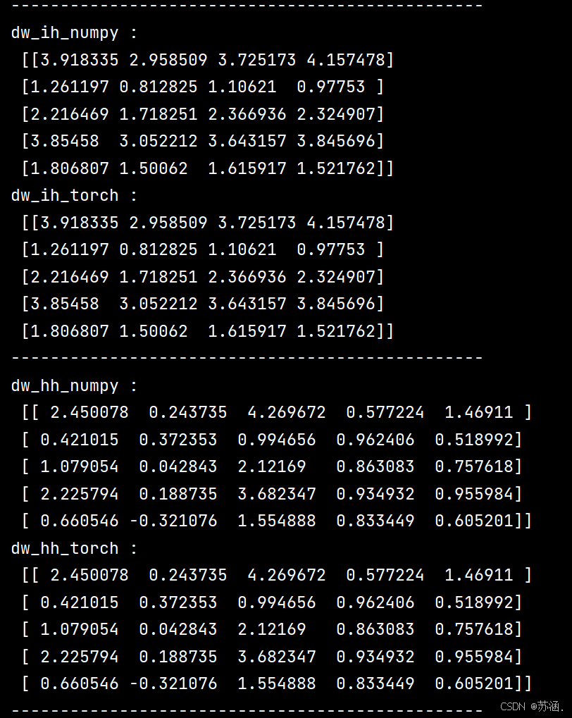
    print("dw_ih_numpy :\n",
          np.sum(rnn_numpy.dw_ih_stack, axis=0))
    print("dw_ih_torch :\n",
          rnn_PyTorch.all_weights[0][0].grad.data.numpy())
    print("------------------------------------------------")

    print("dw_hh_numpy :\n",
          np.sum(rnn_numpy.dw_hh_stack, axis=0))
    print("dw_hh_torch :\n",
          rnn_PyTorch.all_weights[0][1].grad.data.numpy())
    print("------------------------------------------------")

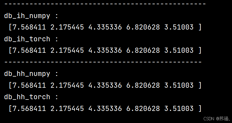
    print("db_ih_numpy :\n",
          np.sum(rnn_numpy.db_ih_stack, axis=(0, 1)))
    print("db_ih_torch :\n",
          rnn_PyTorch.all_weights[0][2].grad.data.numpy())
    print("-----------------------------------------------")
    print("db_hh_numpy :\n",
          np.sum(rnn_numpy.db_hh_stack, axis=(0, 1)))
    print("db_hh_torch :\n",
          rnn_PyTorch.all_weights[0][3].grad.data.numpy())

运行结果：

这次的分享就到这里，下次再见~