- 🍨 本文为 🔗365天深度学习训练营中的学习记录博客
- 🍖 原作者: K同学啊
1.检查GPU
import os,PIL,pathlib,warnings
warnings.filterwarnings("ignore")
device = torch.device("cuda" if torch.cuda.is_available() else "cpu")
device
2.查看数据
import matplotlib.pyplot as plt
plt.rcParams['font.sans-serif'] = ['SimHei']
plt.rcParams['axes.unicode_minus'] = False

import os,PIL,pathlib
data_dir="data/第8天/bird_photos"
data_dir=pathlib.Path(data_dir)

image_count = len(list(data_dir.glob('*/*')))
print("图片总数为:",image_count)
3.划分数据集
python
batch_size = 8
img_height = 224
img_width = 224

import torchvision.transforms as transforms
import torchvision.datasets as datasets
transforms=transforms.Compose([
    transforms.Resize([224,224]),
    transforms.ToTensor(),
    # transforms.Normalize(
    #     mean=[0.482,0.456,0.406],
    #     std=[0.229,0.224,0.225]
    # )
])
total_data=datasets.ImageFolder("data/第8天/bird_photos",transform=transforms)
total_data

total_data.class_to_idx

train_size=int(0.8*len(total_data))
test_size=len(total_data)-train_size
train_data,test_data=torch.utils.data.random_split(total_data,[train_size,test_size])
train_data,test_data

batch_size=8
train_dl=torch.utils.data.DataLoader(train_data,batch_size,shuffle=True,num_workers=1)
test_dl=torch.utils.data.DataLoader(test_data,batch_size,shuffle=True,num_workers=1)

for X,y in train_dl:
    print(X.shape)
    print(y.shape)
    break


4.创建模型
python
import torch
import torch.nn as nn
import torch.nn.functional as F

# ResNet的残差块
class ResBlock(nn.Module):
    def __init__(self, in_channels, out_channels, stride=1):
        super(ResBlock, self).__init__()
        self.conv1 = nn.Conv2d(in_channels, out_channels, kernel_size=3, stride=stride, padding=1)
        self.bn1 = nn.BatchNorm2d(out_channels)
        self.conv2 = nn.Conv2d(out_channels, out_channels, kernel_size=3, stride=1, padding=1)
        self.bn2 = nn.BatchNorm2d(out_channels)
        self.shortcut = nn.Sequential()
        if stride != 1 or in_channels != out_channels:
            self.shortcut = nn.Sequential(
                nn.Conv2d(in_channels, out_channels, kernel_size=1, stride=stride),
                nn.BatchNorm2d(out_channels)
            )

    def forward(self, x):
        out = F.relu(self.bn1(self.conv1(x)))
        out = self.bn2(self.conv2(out))
        out += self.shortcut(x)  # 残差连接
        return F.relu(out)

# DenseNet的密集块
class DenseBlock(nn.Module):
    def __init__(self, in_channels, growth_rate, num_layers):
        super(DenseBlock, self).__init__()
        self.layers = nn.ModuleList()
        for i in range(num_layers):
            self.layers.append(self._make_layer(in_channels + i * growth_rate, growth_rate))

    def _make_layer(self, in_channels, growth_rate):
        return nn.Sequential(
            nn.Conv2d(in_channels, growth_rate, kernel_size=3, padding=1),
            nn.BatchNorm2d(growth_rate),
            nn.ReLU(inplace=True),
            nn.Conv2d(growth_rate, growth_rate, kernel_size=3, padding=1),
            nn.BatchNorm2d(growth_rate)
        )

    def forward(self, x):
        for layer in self.layers:
            new_features = layer(x)
            x = torch.cat([x, new_features], 1)  # DenseNet: 将特征图拼接
        return x

# 混合网络模型
class ResNetDenseNet(nn.Module):
    def __init__(self, in_channels=3, num_classes=1000):
        super(ResNetDenseNet, self).__init__()
        self.conv1 = nn.Conv2d(in_channels, 64, kernel_size=7, stride=2, padding=3)
        self.bn1 = nn.BatchNorm2d(64)
        self.layer1 = ResBlock(64, 64)
        self.dense_block = DenseBlock(64, growth_rate=32, num_layers=4)  # DenseNet模块
        self.fc = nn.Linear(64 + 32 * 4, num_classes)  # 全连接层

    def forward(self, x):
        x = F.relu(self.bn1(self.conv1(x)))
        x = self.layer1(x)  # ResNet残差块
        x = self.dense_block(x)  # DenseNet块
        x = F.adaptive_avg_pool2d(x, (1, 1))  # 全局池化
        x = torch.flatten(x, 1)
        x = self.fc(x)
        return x

model = ResNetDenseNet().to(device)
model


5.编译及训练模型
python
def train(dataloader,model,loss_fn,optimizer):
    size=len(dataloader.dataset)
    num_batches=len(dataloader)
    train_loss,train_acc=0,0
    for X,y in dataloader:
        X,y =X.to(device),y.to(device)
        pred=model(X)
        loss=loss_fn(pred,y)
        #反向传播
        optimizer.zero_grad()
        loss.backward()
        optimizer.step()

        train_loss+=loss.item()
        train_acc+=(pred.argmax(1)==y).type(torch.float).sum().item()
    train_acc/=size
    train_loss/=num_batches
    return train_acc,train_loss
def test(dataloader,model,loss_fn):
    size=len(dataloader.dataset)
    num_batches=len(dataloader)
    test_loss,test_acc=0,0
    with torch.no_grad():
        for imgs,target in dataloader:
            imgs,target=imgs.to(device),target.to(device)
            target_pred=model(imgs)
            loss=loss_fn(target_pred,target)
            test_loss+=loss.item()
            test_acc+=(target_pred.argmax(1)==target).type(torch.float).sum().item()
    test_acc/=size
    test_loss/=num_batches
    return test_acc,test_loss

import copy
optimizer  = torch.optim.Adam(model.parameters(), lr= 1e-4)
loss_fn    = nn.CrossEntropyLoss()

import copy
import torch

# Loss function and other initializations
loss_fn = nn.CrossEntropyLoss()
epochs = 20
train_loss = []
train_acc = []
test_loss = []
test_acc = []
best_acc = 0
best_loss = float('inf')  # 初始化最优损失为正无穷
patience = 5  # 设置耐心值,即连续5轮损失不下降时停止训练
patience_counter = 0  # 用于记录损失不下降的轮数

# Training and testing loop
for epoch in range(epochs):
    model.train()
    epoch_train_acc, epoch_train_loss = train(train_dl, model, loss_fn, optimizer)

    model.eval()
    epoch_test_acc, epoch_test_loss = test(test_dl, model, loss_fn)

    # Check if test loss improved
    if epoch_test_loss < best_loss:
        best_loss = epoch_test_loss
        best_model = copy.deepcopy(model)
        patience_counter = 0  # 重置耐心计数器
    else:
        patience_counter += 1  # 增加耐心计数器

    # If patience is exceeded, stop training
    if patience_counter >= patience:
        print(f"Stopping early at epoch {epoch+1} due to no improvement in test loss for {patience} epochs.")
        break

    train_acc.append(epoch_train_acc)
    train_loss.append(epoch_train_loss)
    test_acc.append(epoch_test_acc)
    test_loss.append(epoch_test_loss)

    # Print the results for the current epoch
    lr = optimizer.state_dict()['param_groups'][0]['lr']
    template = ('Epoch:{:2d}, Train_acc:{:.1f}%, Train_loss:{:.3f}, Test_acc:{:.1f}%, Test_loss:{:.3f}, Lr:{:.2E}')
    print(template.format(epoch + 1, epoch_train_acc * 100, epoch_train_loss,
                          epoch_test_acc * 100, epoch_test_loss, lr))

# Save the best model
PATH = './best_model.pth'
torch.save(best_model.state_dict(), PATH)
print('Finished Training')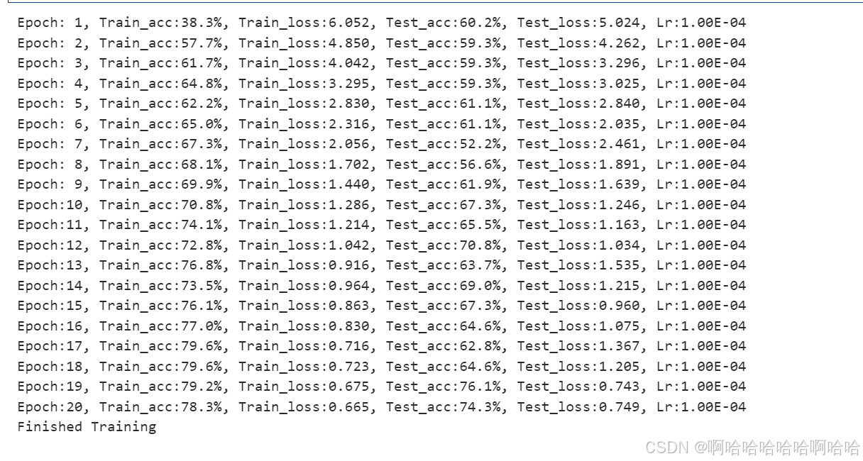
6.结果可视化
python
import matplotlib.pyplot as plt
import warnings
epochs = len(train_acc)

# 绘制准确率
plt.figure(figsize=(12, 6))
plt.subplot(1, 2, 1)
plt.plot(range(1, epochs + 1), train_acc, label='Train Accuracy', color='blue')
plt.plot(range(1, epochs + 1), test_acc, label='Test Accuracy', color='orange')
plt.title('Training and Test Accuracy')
plt.xlabel('Epochs')
plt.ylabel('Accuracy')
plt.legend(loc='best')

# 绘制损失
plt.subplot(1, 2, 2)
plt.plot(range(1, epochs + 1), train_loss, label='Train Loss', color='blue')
plt.plot(range(1, epochs + 1), test_loss, label='Test Loss', color='orange')
plt.title('Training and Test Loss')
plt.xlabel('Epochs')
plt.ylabel('Loss')
plt.legend(loc='best')

# 显示图形
plt.tight_layout()
plt.show()
7.预测图片
python
import os,PIL,random,pathlib

data_dir='data/第8天/bird_photos'
data_path=pathlib.Path(data_dir)
data_paths=list(data_path.glob('*'))
classNames=[str(path).split('\\')[3] for path in data_paths]
classNames

print(images[i].shape)

plt.figure(figsize=(10, 5))
plt.suptitle("Photo Predictions")

for images, labels in test_dl:
    for i in range(min(8, len(images))):
        ax = plt.subplot(2, 4, i + 1)

        img_tensor = images[i]

        # 如果img_tensor不是numpy数组或者没有归一化到[0, 1],先进行转换
        img_array = img_tensor.squeeze().permute(1, 2, 0).cpu().numpy()
        if img_array.min() < 0 or img_array.max() > 1:
            img_array = (img_array - img_array.min()) / (img_array.max() - img_array.min())

        plt.imshow(img_array)

        model.eval()
        with torch.no_grad():
            predictions = model(img_tensor.unsqueeze(0).to(device))
            predicted_label = classNames[predictions.argmax(dim=1).item()]

        plt.title(predicted_label)
        plt.axis("off")
    break
plt.show() 总结:
总结:
1.创新点:
-
结合 ResNet 和 DenseNet:充分利用两种网络的优点,提取更丰富的特征。
-
混合特征提取:通过残差块和密集块的组合,增强特征表示能力。
-
特征重用:通过密集连接实现特征重用,提高参数效率。
-
全局池化:减少参数量,避免全连接层对输入尺寸的依赖。
-
灵活性和可扩展性:模型结构灵活,可以根据任务需求进行调整。
-
模型结构:
pythonimport torchsummary as summary summary.summary(model, (3, 224, 224))

2.早停机制:
python
import copy
import torch

# Loss function and other initializations
loss_fn = nn.CrossEntropyLoss()
epochs = 20
train_loss = []
train_acc = []
test_loss = []
test_acc = []
best_acc = 0
best_loss = float('inf')  # 初始化最优损失为正无穷
patience = 5  # 设置耐心值,即连续5轮损失不下降时停止训练
patience_counter = 0  # 用于记录损失不下降的轮数

# Training and testing loop
for epoch in range(epochs):
    model.train()
    epoch_train_acc, epoch_train_loss = train(train_dl, model, loss_fn, optimizer)

    model.eval()
    epoch_test_acc, epoch_test_loss = test(test_dl, model, loss_fn)

    # Check if test loss improved
    if epoch_test_loss < best_loss:
        best_loss = epoch_test_loss
        best_model = copy.deepcopy(model)
        patience_counter = 0  # 重置耐心计数器
    else:
        patience_counter += 1  # 增加耐心计数器

    # If patience is exceeded, stop training
    if patience_counter >= patience:
        print(f"Stopping early at epoch {epoch+1} due to no improvement in test loss for {patience} epochs.")
        break

    train_acc.append(epoch_train_acc)
    train_loss.append(epoch_train_loss)
    test_acc.append(epoch_test_acc)
    test_loss.append(epoch_test_loss)

    # Print the results for the current epoch
    lr = optimizer.state_dict()['param_groups'][0]['lr']
    template = ('Epoch:{:2d}, Train_acc:{:.1f}%, Train_loss:{:.3f}, Test_acc:{:.1f}%, Test_loss:{:.3f}, Lr:{:.2E}')
    print(template.format(epoch + 1, epoch_train_acc * 100, epoch_train_loss,
                          epoch_test_acc * 100, epoch_test_loss, lr))

# Save the best model
PATH = './best_model.pth'
torch.save(best_model.state_dict(), PATH)
print('Finished Training')
3.流程总结:
1. 代码结构
代码分为以下几个部分:
-
检查 GPU:检查是否有可用的 GPU,并将模型和数据加载到 GPU 上。
-
查看数据:加载数据集并统计图片数量。
-
划分数据集:将数据集划分为训练集和测试集,并创建数据加载器。
-
创建模型 :定义了一个结合 ResNet 和 DenseNet 的混合模型。
-
编译及训练模型:定义了训练和测试函数,并进行了模型训练。
-
结果可视化:绘制训练和测试的准确率和损失曲线。
-
预测图片:对测试集中的图片进行预测,并可视化预测结果。
2. 模型设计
模型的核心是一个结合 ResNet 和 DenseNet 的混合网络:
-
ResNet 残差块:通过残差连接解决了梯度消失问题,使得网络可以训练得更深。
-
DenseNet 密集块:通过密集连接实现了特征重用,提高了参数效率。
-
混合模型 :先通过一个 ResNet 残差块 提取特征,然后通过一个 DenseNet 密集块 进一步提取和重用特征,最后通过全局平均池化和全连接层进行分类。
3. 数据集处理
-
数据集被划分为训练集和测试集,比例为 80% 和 20%。
-
数据加载器使用了
torch.utils.data.DataLoader,支持批量加载和数据打乱。 -
数据预处理包括调整大小 (
Resize) 和转换为张量 (ToTensor)。
4. 训练和测试
-
训练函数:计算损失并进行反向传播,更新模型参数。
-
测试函数:在测试集上评估模型性能,计算准确率和损失。
-
早停机制:如果测试损失在连续 5 轮训练中没有下降,则提前停止训练。
-
模型保存:保存测试损失最小的模型。
5. 结果可视化
-
绘制了训练和测试的准确率和损失曲线,直观展示了模型的性能。
-
准确率曲线反映了模型在训练集和测试集上的分类能力。
-
损失曲线反映了模型在训练集和测试集上的优化情况。
6. 预测图片
-
对测试集中的图片进行预测,并可视化预测结果。
-
预测结果以图片标题的形式显示,便于观察模型的分类效果。