决策树（Decision Tree）案例分析

Iris鸢尾花分类

数据概况
导入函数库
读取数据
- 数据清洗
探索性数据分析（EDA）
特征工程
模型选择&训练
结果分析
算法优化
- 1、解决过拟合问题：手动调节参数
- [2、10折交叉验证 for 决策树超参数调优](#2、10折交叉验证 for 决策树超参数调优)
- 3、后剪枝
- 4、只有后2维特征是重要的，在2D平面上可视化决策边界

数据概况

导入函数库

go 复制代码

import pandas as pd
import numpy as np

from sklearn.tree import DecisionTreeClassifier
from sklearn.model_selection import GridSearchCV

from sklearn.metrics import accuracy_score
from sklearn.metrics import roc_auc_score

#作图
import matplotlib.pyplot as plt 
%matplotlib inline

#显示中文
plt.rcParams['font.sans-serif'] = ['Arial Unicode MS']

读取数据

go 复制代码

#读取数据
# csv文件没有列名，增加列名：花萼长度、宽度；花瓣长度、宽度
feat_names = ['sepal-length', 'sepal-width', 'petal-length', 'petal-width']
col_names = feat_names + ['species']

dpath = ""
df = pd.read_csv(dpath + "iris.csv", names = col_names)

#通过观察前5行，了解数据每列（特征）的概况
df.head()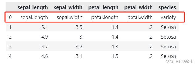

数据清洗

发现第一行奇奇怪怪的，是垃圾（冗余/无用）数据，我们直接删掉。

go 复制代码

# 删除第1行
df = df.drop(index=0)  # 删除索引为 0 的行（第 1 行）
df.head()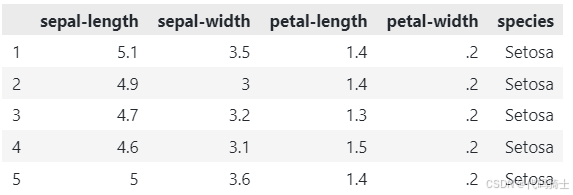

舒服了。

探索性数据分析（EDA）

查看整体数据信息

go 复制代码

# 数据总体信息
df.info()

竟然全是object类型，没有数值型，显然后面我们要进行数据类型转换。

查看基本统计值

go 复制代码

df.describe()

特征之间差距不大，不太需要标准化。

检查缺失值

go 复制代码

print(df.isnull().any())
print(df.isnull().sum())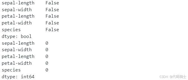

一个缺失值都没得。

也可以用可视化的方式查看缺失值。

go 复制代码

import missingno as msno
# 矩阵图
msno.matrix(df)
plt.show()

# 条形图
msno.bar(df)
plt.show()

# 热力图
msno.heatmap(df)
plt.show()

# 树状图
msno.dendrogram(df)
plt.show()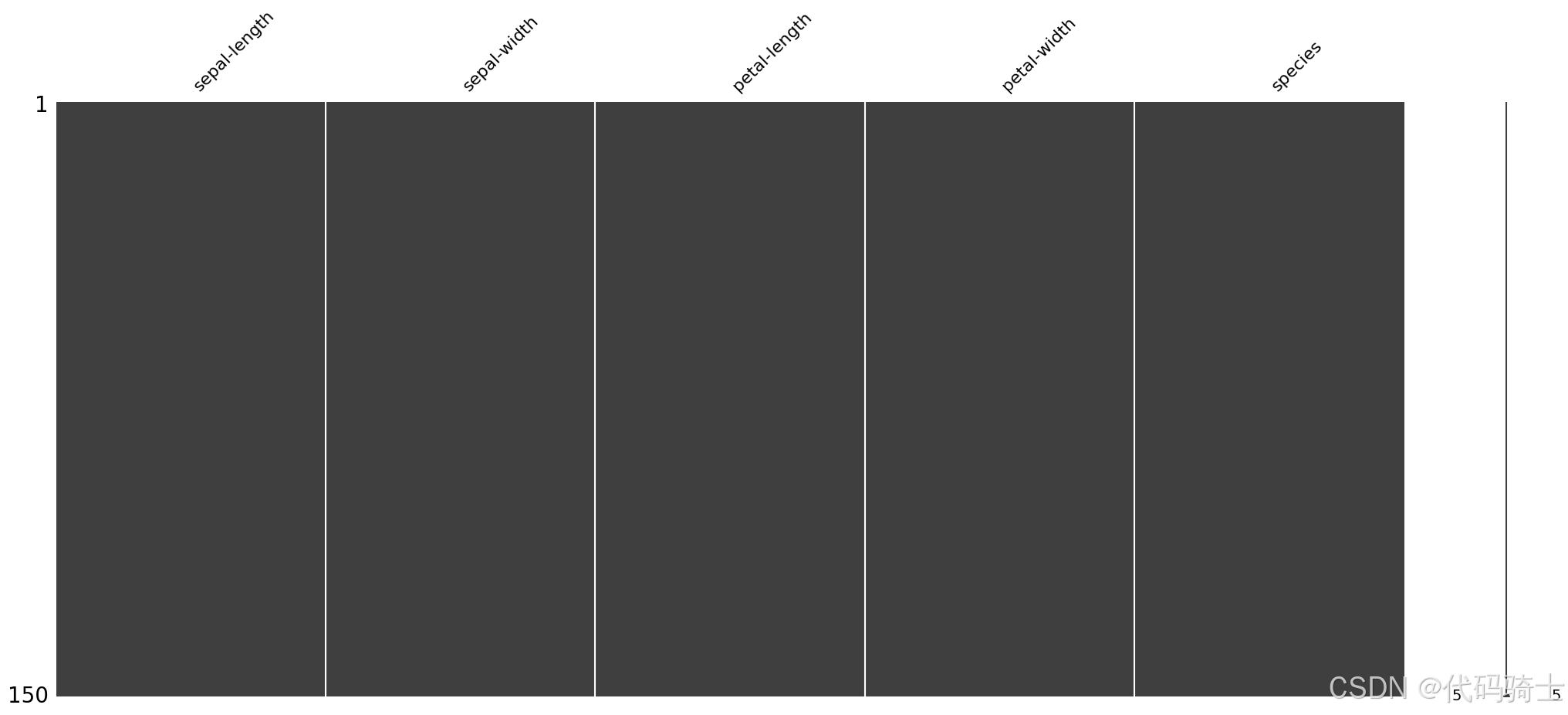

特征工程

特征编码

查看种类值：

go 复制代码

df['species'].value_counts()

将三个种类对应三个数值编码012。

go 复制代码

#标签字符串映射为整数（在此并不一定需要）
target_map = {'Setosa':0, 
              'Versicolor':1,
              'Virginica':2 }  #2

# Use the pandas apply method to numerically encode our attrition target variable
df['species'] = df['species'].apply(lambda x: target_map[x])

更优雅的写法：

go 复制代码

df['species'] = df['species'].map({'Setosa':0,'Versicolor':1,'Virginica':2})

现在类别里全是数字012

go 复制代码

df['species'].values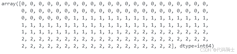

特征提取

go 复制代码

# 从原始数据中分离输入特征x和输出y
y = df['species']
X = df.drop('species', axis = 1)

特征缩放

go 复制代码

# 决策树算法无需特征缩放

切分数据集

go 复制代码

#将数据分割训练数据与测试数据
from sklearn.model_selection import train_test_split

# 随机采样20%的数据构建验证集，其余作为训练样本
X_train, X_test, y_train, y_test = train_test_split(X, y, random_state=42, test_size=0.2, stratify=y)

模型选择&训练

默认使用决策树模型

go 复制代码

clf = DecisionTreeClassifier()

clf.fit(X_train, y_train)

acc_train = clf.score(X_train, y_train)
acc_test = clf.score(X_test, y_test)
print('acc on train: ', acc_train)
print('acc on test: ', acc_test)

acc on train: 1.0

acc on test: 0.9333333333333333

从模型输出来看，训练集的准确率达到了 1.0，这表明模型在训练集上表现完美。然而，这可能是一个过拟合的迹象，尤其是当测试集的准确率远低于训练集时。

go 复制代码

depth = clf.get_depth()
n_leaves = clf.get_n_leaves()
print(depth,n_leaves)

5 8

结果分析

go 复制代码

#从scikit-learn 版本21.0开始，可以使用scikit-learn的tree.plot_tree方法,利用matplotlib将决策树可视化
from sklearn import tree

class_names =['setosa', 'versicolor', 'virginica']

plt.figure(figsize=(20,20)) 
a = tree.plot_tree(clf,
                   feature_names = feat_names,
                   class_names = class_names)
plt.show()

决策树图像

这个图像是一个决策树的可视化图，展示了决策树的结构和决策路径。图中每个节点包含以下信息：

分裂特征：用于分裂数据的特征名称（例如 petal-width）。
分裂阈值：用于分裂数据的阈值（例如 <= 0.8）。
Gini系数：衡量节点不纯度的指标，值越小表示节点越纯。
样本数：节点包含的样本数量。
类别分布：节点中各类别的样本数量（例如 [40, 40, 40]）。
预测类别：节点的预测类别。

go 复制代码

x = range(len(feat_names))
plt.bar(x, clf.feature_importances_)
plt.xticks(x, feat_names)
plt.show()

特征重要性图

这个图像是一个条形图，展示了各个特征的重要性。图中每个条形的高度表示对应特征的重要性值，值越大表示该特征对模型预测的贡献越大。从图中可以看出，petal-width 特征的重要性远高于其他特征，说明它对模型的预测能力贡献最大。其次是 petal-length，然后是 sepal-width，最后是 sepal-length。

算法优化

1、解决过拟合问题：手动调节参数

解决方法：

限制决策树的深度：可以通过设置 max_depth 参数来控制决策树的最大深度。
限制叶节点数量：可以通过设置 max_leaf_nodes 参数来限制叶节点的数量。
最小样本分割：通过设置 min_samples_split 参数，确保每个节点至少有指定数量的样本才能分裂。
最小样本叶子节点：通过设置 min_samples_leaf 参数，确保每个叶子节点至少有指定数量的样本。

go 复制代码

from sklearn.tree import DecisionTreeClassifier

# 设置限制参数
clf = DecisionTreeClassifier(max_depth=3, min_samples_split=2, min_samples_leaf=1)
clf.fit(X_train, y_train)

acc_train = clf.score(X_train, y_train)
acc_test = clf.score(X_test, y_test)
print('acc on train: ', acc_train)
print('acc on test: ', acc_test)

acc on train: 0.9833333333333333

acc on test: 0.9666666666666667

2、10折交叉验证 for 决策树超参数调优

max_depth（树的深度）或max_leaf_nodes（叶子结点的数目）、
min_samples_leaf（叶子结点的最小样本数）、min_samples_split（中间结点的最小样本树）、min_weight_fraction_leaf（叶子节点的样本权重占总权重的比例）
min_impurity_split（最小不纯净度）也可以调整

这个数据集的任务不难，深度设为1-8之间

go 复制代码

from sklearn.model_selection import GridSearchCV

#设置超参数搜索范围
max_depth = range(2,8,1)
min_samples_leaf = range(1,7,1)
tuned_parameters = dict(max_depth=max_depth, min_samples_leaf=min_samples_leaf)

#生成学习器实例
clf = DecisionTreeClassifier()

#生成GridSearchCV实例
grid= GridSearchCV(clf, tuned_parameters, cv=10, scoring='accuracy',n_jobs = 4, verbose=1)

#训练，交叉验证对超参数调优
grid.fit(X_train, y_train)

go 复制代码

print("Best: %f using %s" % (grid.best_score_, grid.best_params_))

上述代码可能因为配置原因跑不出来，修改成下面的简易版，cv=3折

go 复制代码

from sklearn.model_selection import GridSearchCV
from sklearn.tree import DecisionTreeClassifier

max_depth = range(2, 5)
min_samples_leaf = range(1, 4)
tuned_parameters = dict(max_depth=max_depth, min_samples_leaf=min_samples_leaf)

clf = DecisionTreeClassifier()

grid = GridSearchCV(clf, tuned_parameters, cv=3, scoring='accuracy', n_jobs=1, verbose=1, pre_dispatch="2*n_jobs")

if __name__ == "__main__":
    grid.fit(X_train, y_train)
    print("Best Parameters:", grid.best_params_)

Fitting 3 folds for each of 9 candidates, totalling 27 fits

Best Parameters: {'max_depth': 4, 'min_samples_leaf': 1}

go 复制代码

test_means = grid.cv_results_[ 'mean_test_score' ]
test_means

array([0.93333333, 0.93333333, 0.93333333, 0.95833333, 0.95833333,

0.95833333, 0.96666667, 0.95 , 0.95833333])

go 复制代码

test_means = grid.cv_results_[ 'mean_test_score' ]

# plot results
test_scores = np.array(test_means).reshape(len(max_depth), len( min_samples_leaf))

for i, value in enumerate(max_depth):
    plt.plot(min_samples_leaf, test_scores[i], label= 'max_depth:'   + str(value))

    
plt.legend()
plt.xlabel( 'min_samples_leaf' )                                                                                                      
plt.ylabel( 'accuraccy' )
plt.show()

go 复制代码

clf = grid.best_estimator_

acc_train = clf.score(X_train, y_train)
acc_test = clf.score(X_train, y_train)
print('acc on train: ', acc_train)
print('acc on test: ', acc_test)

acc on train: 0.9916666666666667

acc on test: 0.9916666666666667

go 复制代码

plt.figure(figsize=(10,8)) 

fig = tree.plot_tree(clf,
                   feature_names = feat_names,
                   class_names = class_names)
plt.show()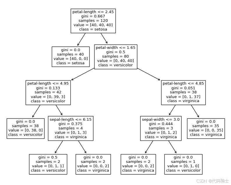

数据有较小的变化，得到的决策树差异很大。所以决策树模型的方差大

go 复制代码

x = range(len(feat_names))
plt.bar(x, clf.feature_importances_)
plt.xticks(x, feat_names)
plt.show()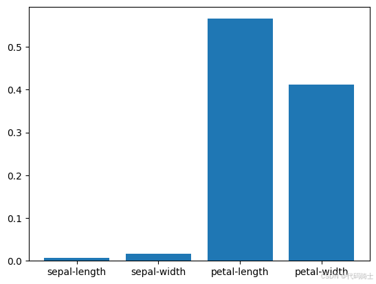

3、后剪枝

go 复制代码

path = clf.cost_complexity_pruning_path(X_train, y_train)
ccp_alphas, impurities = path.ccp_alphas, path.impurities
clfs = []
for ccp_alpha in ccp_alphas:
     clf = DecisionTreeClassifier(random_state=0, ccp_alpha=ccp_alpha)
     clf.fit(X_train, y_train)
     clfs.append(clf)

train_scores = [clf.score(X_train, y_train) for clf in clfs]
test_scores = [clf.score(X_test, y_test) for clf in clfs]

fig, ax = plt.subplots()
ax.set_xlabel("alpha")
ax.set_ylabel("accuracy")
ax.set_title("Accuracy vs alpha for training and testing sets")
ax.plot(ccp_alphas, train_scores, marker="o", label="train", drawstyle="steps-post")
ax.plot(ccp_alphas, test_scores, marker="o", label="test", drawstyle="steps-post")
ax.legend()
plt.show()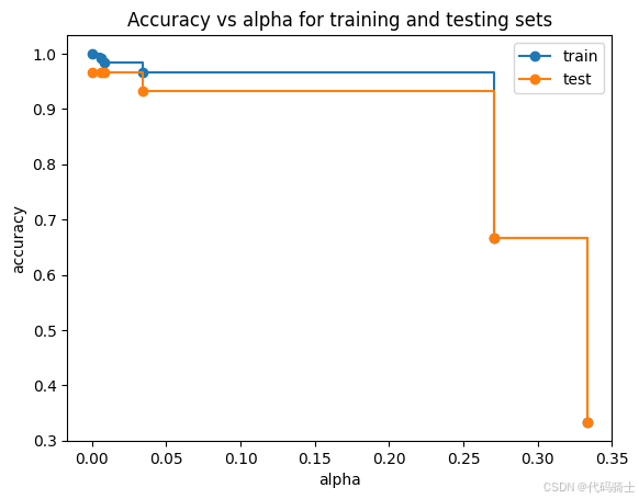

取test最好的alpha为0.0，即不需要后剪枝。

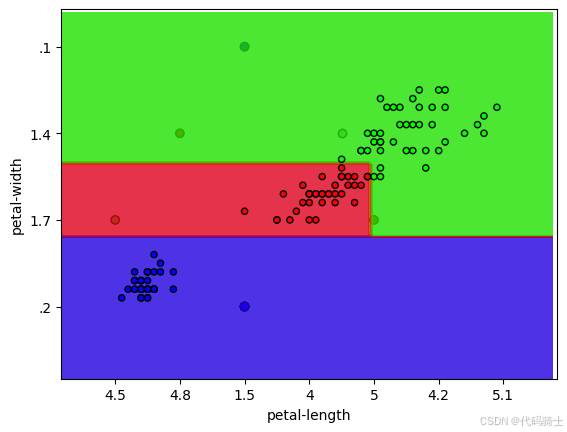
4、只有后2维特征是重要的，在2D平面上可视化决策边界

go 复制代码

X_train_2d = np.array(X_train.loc[:, ['petal-length', 'petal-width']]) 
X_test_2d = np.array(X_test.loc[:, ['petal-length', 'petal-width']])

go 复制代码

clf = DecisionTreeClassifier(max_depth = 3, min_samples_leaf = 3)
clf.fit(X_train_2d, y_train)

go 复制代码

import numpy as np
import matplotlib.pyplot as plt

def plot_2d_separator(clf, X, ax=None):
    # 确保 X 是数值类型
    X = np.array(X, dtype=np.float64)
    
    eps = X.std() / 2.
    x1_min, x2_min = X.min(axis=0) - eps
    x1_max, x2_max = X.max(axis=0) + eps
    x1_range = np.arange(x1_min, x1_max, (x1_max - x1_min) / 100)
    x2_range = np.arange(x2_min, x2_max, (x2_max - x2_min) / 100)
    x1, x2 = np.meshgrid(x1_range, x2_range)

    # 预测整个网格的类别
    Z = clf.predict(np.c_[x1.ravel(), x2.ravel()])
    Z = Z.reshape(x1.shape)

    if ax is None:
        ax = plt.gca()
    ax.contourf(x1, x2, Z, alpha=0.8, cmap=plt.cm.brg)
    ax.scatter(X[:, 0], X[:, 1], c=clf.predict(X), cmap=plt.cm.brg, edgecolors='k', s=20)
    ax.set_xlim(x1_min, x1_max)
    ax.set_ylim(x2_min, x2_max)

go 复制代码

plt.scatter(X_train_2d[:, 0], X_train_2d[:, 1], c = y_train, cmap=plt.cm.brg,marker='o', edgecolors='k')
plt.scatter(X_test_2d[:, 0], X_test_2d[:, 1], c = y_test, cmap=plt.cm.brg,marker='o', edgecolors='k')
plt.scatter(4.5, 2.0, c = '#A9A9A9', marker='o', edgecolors='k')  #darkgray, query

plot_2d_separator(clf, X_train_2d) # plot the boundary

plt.xlabel('petal-length')
plt.ylabel('petal-width')
#plt.xlabel(u'花萼长度')
#plt.ylabel(u'花萼宽度')
#plt.legend()
plt.show()