实验三用Tensorflow构建神经网络实现激酶抑制剂分类

一、问题描述

激酶抑制剂是一种抑制激酶活性的化合物。蛋白激酶用于调节细胞的多个功能，自2001年以来已有76种激酶抑制剂获批上市，例如伊马替尼（Imatinib）已被成功应用于癌症治疗。这里使用的数据集为包含2013个激酶抑制剂的四分类数据，每个数据包含5个特征。

二、解决方案

采用神经网络算法对激酶抑制剂进行分类。神经网络是一种模拟人脑神经元工作原理的机器学习算法，广泛用于分类、回归和特征提取等任务。这里使用Python的sklearn库来构建和训练神经网络模型，并对模型的结果进行分析。

三、实验步骤

神经网络的实现流程一般分为4部分：数据预处理、神经网络构建、模型训练和模型使用。

1、数据准备

数据收集：获取包含激酶抑制剂的化合物特征和标签的数据集。

数据清理：检查缺失值、异常值并进行处理。

2、数据预处理

特征选择：选择合适的特征用于模型训练。

数据标准化：对特征进行标准化处理，常用的方法是 Min-Max Scaling 或 Z-score 标准化。

划分数据集：将数据划分为训练集和测试集。

3、构建神经网络模型

使用 TensorFlow/Keras 构建神经网络。

4、训练模型

训练模型并监控训练过程中的损失和准确性。

5、评估模型

使用测试集评估模型的性能。

6、可视化结果

绘制训练过程中的损失和准确性曲线。

7、模型预测

对新样本进行预测。

8、保存模型

在训练完成后，可以将模型保存以便后续使用。

四、核心代码

python 复制代码

# In[330]:
from sklearn.model_selection import train_test_split
from sklearn.preprocessing import StandardScaler,LabelEncoder

import pandas as pd
import numpy as np

# In[331]:
dataframe = pd.read_csv("kinase_selected.csv")
dataframe.head()


# In[340]:
dataset = dataframe.values#不含属性标签的数据值列表
X = dataset[:, 1:]

scaler = StandardScaler()#定义标准化方法对象
X_scaled = scaler.fit_transform(X)#将数据传入标准化方法对象中，进行标准化处理
print('X_scaled.shape:',X_scaled.shape)

feature_names = dataframe.columns.values[1:]
features = np.array(feature_names)
print("All features:\n",features)
print("length of features", len(features))


# In[387]:
label = pd.read_csv('label_kinase_selected.csv' )
label.head()
y = label.iloc[:, -1]
print('y.shape:',y.shape)
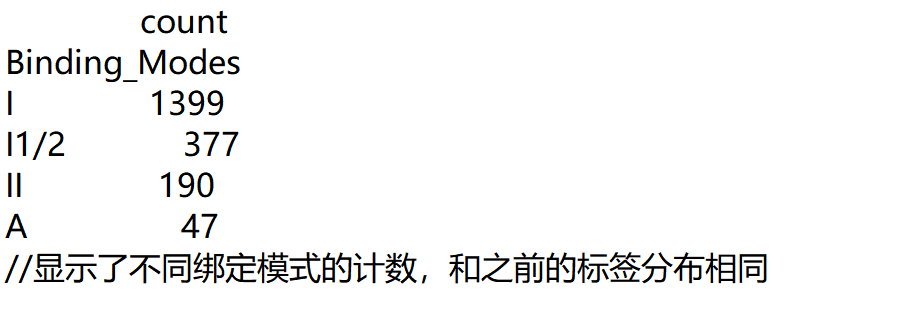
pd.DataFrame(label['Binding_Modes'].value_counts())


# In[389]:
from tensorflow import keras
le = LabelEncoder()
# lable encoder
Y = le.fit_transform(y)
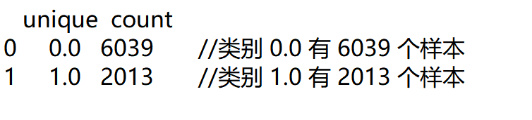
unique,count=np.unique(tuple(Y),return_counts=True)
print(pd.DataFrame({'unique':unique,'label':le.inverse_transform([0,1,2,3]),'count':count}))
unique = keras.utils.to_categorical(unique)
print('unique_encoder:\n',unique)  # 数字代表第x个标签
Y = keras.utils.to_categorical(Y)
print(pd.DataFrame(label['Binding_Modes'].value_counts()))  # 获得各标签的数量

# split into input (X) and output (Y) variables
X_train, X_test, Y_train, Y_test = train_test_split(
    X_scaled, Y, test_size=0.2, random_state=42, stratify=Y)

print("Feature data dimension: ", X_train.shape)
print("Num of classes: ", Y_train.shape[1])


# In[379]:
label['Binding_Modes'].value_counts().name


# In[367]:
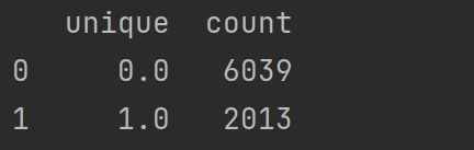
unique,count=np.unique(tuple(Y),return_counts=True)
print(pd.DataFrame({'unique':unique,'count':count}))

# #### 搭建神经网络
# In[314]:
from keras.layers import Dense, Dropout
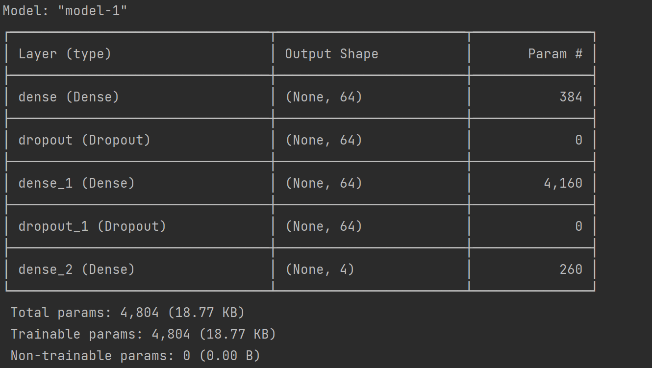
model = keras.Sequential(name='model-1')
model.add(Dense(64, activation='relu', input_shape=(5,)))
model.add(Dropout(0.2))
model.add(Dense(64, activation='relu'))
model.add(Dropout(0.2))
model.add(Dense(4, activation='softmax'))
model.summary()


# #### 设置模型优化器、损失函数、评价指标

# In[315]:
model.compile(optimizer='adam',
              loss='categorical_crossentropy',
              metrics=['accuracy']
              )


# #### 开始训练

# In[317]:
history = model.fit(X_train, Y_train,
                    batch_size=16,
                    epochs=1000
                    )


# #### 用测试数据进行数据预测，并与实际的结果进行误差百分比的计算

# In[318]:
Y_test

# In[319]:
y_predict = model.predict(X_test)
y_predict


# In[320]
y_predict[0]


# In[321]:
y_predict_label = [np.argmax(i) for i in y_predict]
# y_test_label = [np.argmax(i) for i in Y_train]
y_test_label = [np.argmax(i) for i in Y_test]
print(y_predict_label)
print(y_test_label)


# In[322]:
correct_prediction = np.equal(y_predict_label, y_test_label)
print(np.mean(correct_prediction))


# In[323]:
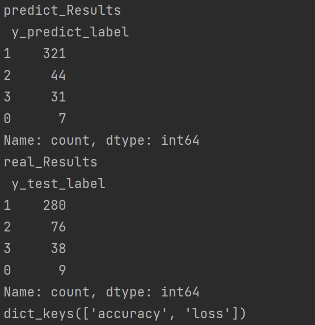
# pd.DataFrame({'y_predict_label':y_predict_label,'y_test_label':y_test_label}).value_counts()
print("predict_Results\n", pd.DataFrame(
    {'y_predict_label': y_predict_label})['y_predict_label'].value_counts())
print("real_Results\n", pd.DataFrame(
    {'y_test_label': y_test_label})['y_test_label'].value_counts())


# In[324]:
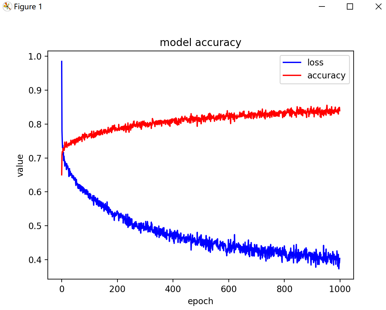
import matplotlib.pyplot as plt
print(history.history.keys())
plt.plot(history.history['loss'], 'b')
plt.plot(history.history['accuracy'], 'r')
plt.title("model accuracy")
plt.ylabel("value")
plt.xlabel("epoch")
plt.legend(["loss", "accuracy"])
plt.show()
print('loss--------',history.history['loss'][-1])
print('accuracy----',history.history['accuracy'][-1])


# In[325]:
plt.rcParams['font.sans-serif'] = ['SimHei']  # 用来正常显示中文标签
plt.rcParams['axes.unicode_minus'] = False  # 用来正常显示负号

plt.scatter(X_test[:, 0], X_test[:, 3],
            c=y_predict_label, marker='o')
plt.xlabel('指标1')
plt.ylabel('指标2')
plt.title('类型分布')
plt.show()