探索大语言模型（LLM）：马尔可夫链——从诗歌分析到人工智能的数学工具

提出背景与灵感起源

马尔可夫链由俄国数学家安德雷·马尔可夫 于1906年提出，最初是为了挑战当时概率论中"独立性假设"的局限性。他希望通过研究相依变量序列 ，证明即使随机变量之间存在依赖关系，大数定律和中心极限定理仍然成立。 灵感来源：马尔可夫在1913年分析了普希金的长诗《叶甫盖尼·奥涅金》，统计了元音和辅音字母的交替规律。他发现字母序列的统计特性可以用一种"当前状态仅依赖前一步"的模型描述，这成为马尔可夫链的雏形。这种将语言结构与概率结合的方法，揭示了随机过程中的有序性。

数学定义与公式推导

1. 马尔可夫性质

核心定义 ：若随机过程满足 <math xmlns="http://www.w3.org/1998/Math/MathML"> P ( X t + 1 = x ∣ X 0 , X 1 , . . . , X t ) = P ( X t + 1 = x ∣ X t ) P(X_{t+1}=x | X_0, X_1, ..., X_t) = P(X_{t+1}=x | X_t) </math>P(Xt+1=x∣X0,X1,...,Xt)=P(Xt+1=x∣Xt) 则称其具有马尔可夫性质 ，即"未来仅取决于现在，与过去无关"。只依赖于当前状态，这种特性被称为 "无记忆性" 或 "马尔科夫性"。

2. 转移概率矩阵

假设状态空间为 <math xmlns="http://www.w3.org/1998/Math/MathML"> S = { s 1 , s 2 , . . . , s n } S = \{s_1, s_2, ..., s_n\} </math>S={s1,s2,...,sn}，定义单步转移概率：
<math xmlns="http://www.w3.org/1998/Math/MathML"> P i j = P ( X t + 1 = s j ∣ X t = s i ) P_{ij} = P(X_{t+1}=s_j | X_t = s_i) </math>Pij=P(Xt+1=sj∣Xt=si)

则转移矩阵为：
<math xmlns="http://www.w3.org/1998/Math/MathML"> P = [ P 11 P 12 ⋯ P 1 n P 21 P 22 ⋯ P 2 n ⋮ ⋮ ⋱ ⋮ P n 1 P n 2 ⋯ P n n ] P = \begin{bmatrix}P_{11} & P_{12} & \cdots & P_{1n} \\P_{21} & P_{22} & \cdots & P_{2n} \\\vdots & \vdots & \ddots & \vdots \\P_{n1} & P_{n2} & \cdots & P_{nn}\end{bmatrix} </math>P= P11P21⋮Pn1P12P22⋮Pn2⋯⋯⋱⋯P1nP2n⋮Pnn

矩阵每行元素和为1，即 <math xmlns="http://www.w3.org/1998/Math/MathML"> ∑ j = 1 n P i j = 1 \sum_{j=1}^n P_{ij} = 1 </math>∑j=1nPij=1。

3. 平稳分布

若存在概率分布 <math xmlns="http://www.w3.org/1998/Math/MathML"> π \pi </math>π 满足： <math xmlns="http://www.w3.org/1998/Math/MathML"> π P = π \pi P = \pi </math>πP=π 则称 <math xmlns="http://www.w3.org/1998/Math/MathML"> π \pi </math>π 为平稳分布。通过求解线性方程组可得到长期状态下的稳定概率。

4.公式推导

用转移概率矩阵 <math xmlns="http://www.w3.org/1998/Math/MathML"> P = ( p i j ) P=(p_{ij}) </math>P=(pij)来描述状态之间的转移，其中 <math xmlns="http://www.w3.org/1998/Math/MathML"> p i j = P ( X n + 1 = j ∣ X n = i ) p_{ij}=P(X {n+1}=j∣X_n=i) </math>pij=P(Xn+1=j∣Xn=i)，表示从状态i转移到状 j的一步转移概率，且满足 <math xmlns="http://www.w3.org/1998/Math/MathML"> ∑ j ∈ S p i j = 1 \sum\limits{j∈S}p_{ij}=1 </math>j∈S∑pij=1，因为从状态i出发，下一步必然转移到状态空间S中的某个状态。

对于n步转移概率，记为 <math xmlns="http://www.w3.org/1998/Math/MathML"> p i j ( n ) = P ( X n + m = j ∣ X m = i ) p_{ij}^{(n)}=P(X_{n+m} =j∣X_m=i) </math>pij(n)=P(Xn+m=j∣Xm=i)，它满足切普曼 - 柯尔莫哥洛夫方程: <math xmlns="http://www.w3.org/1998/Math/MathML"> p i j ( n + m ) = ∑ k ∈ S p i k ( n ) p k j ( m ) p_{ij}^{(n+m)} =\sum\limits_{k∈S} p_{ik}^{(n)}p_{kj}^{(m)} </math>pij(n+m)=k∈S∑pik(n)pkj(m)

推导过程如下：
<math xmlns="http://www.w3.org/1998/Math/MathML" display="block"> p i j ( n + m ) = P ( X n + m = j ∣ X 0 = i ) = ∑ k ∈ S P ( X n + m = j , X n = k ∣ X 0 = i ) ( 全概率公式 ) = ∑ k ∈ S P ( X n + m = j ∣ X n = k , X 0 = i ) ⋅ P ( X n = k ∣ X 0 = i ) ( 条件概率公式 ) = ∑ k ∈ S P ( X n + m = j ∣ X n = k ) ⋅ P ( X n = k ∣ X 0 = i ) = ∑ k ∈ S = p k j ( m ) p i k ( n ) ( 马尔科夫性 ) p_{ij}^{(n+m)}=P(X_{n+m}=j∣X_0=i) \\ \ = \sum\limits_{k∈S}P(X_{n+m}=j,X_n=k∣X_0=i) \ {(全概率公式) }\\ \ = \sum\limits_{k∈S}P(X_{n+m}=j∣X_n=k,X_0=i)⋅P(X_n=k∣X_0=i) \ {(条件概率公式)}\\ \ =\sum\limits_{k∈S}P(X_{n+m}=j∣X_n=k)⋅P(X_n=k∣X_0=i) \\ \ = \sum\limits_{k∈S} \ = p_{kj}^{(m)}p_{ik}^{(n)} (马尔科夫性) </math>pij(n+m)=P(Xn+m=j∣X0=i) =k∈S∑P(Xn+m=j,Xn=k∣X0=i) (全概率公式) =k∈S∑P(Xn+m=j∣Xn=k,X0=i)⋅P(Xn=k∣X0=i) (条件概率公式) =k∈S∑P(Xn+m=j∣Xn=k)⋅P(Xn=k∣X0=i) =k∈S∑ =pkj(m)pik(n)(马尔科夫性)

该方程表明，从状态i经过n+m步转移到状态j的概率，可以通过从状态i先经过n步转移到中间状态k，再从状态k经过m步转移到状态j，然后对所有可能的中间状态k求和得到。

这为计算多步转移概率提供了递归的方法，也使得我们能够通过一步转移概率矩阵的幂运算来计算任意步的转移概率。

通俗示例

例1:早餐选择

早餐选择模型假设小明每天早餐在A（包子）和B（煎饼）之间选择，规则如下：

若今天选A，明天选A的概率40%，选B的概率60%
若今天选B，明天选A和B的概率各50%

转移矩阵 ：
<math xmlns="http://www.w3.org/1998/Math/MathML"> P = [ 0.4 0.6 0.5 0.5 ] P = \begin{bmatrix}0.4 & 0.6 \\0.5 & 0.5\end{bmatrix} </math>P=[0.40.50.60.5] 转移矩阵对应转移状态示意图

代码模拟10天早餐序列：

python 复制代码

import numpy as np
# 定义转移矩阵和初始状态
P = [[0.4, 0.6], [0.5, 0.5]]
current_state = 0  # 初始状态为A
states = ['A', 'B']  # 模拟状态转移
np.random.seed(42)
for _ in range(10):    
	print(f"Day {_+1}: {states[current_state]}")    
	current_state = np.random.choice([0,1], p=P[current_state])

输出结果：

less 复制代码

Day 1: A
Day 2: B
Day 3: A
Day 4: B
Day 5: A
Day 6: B
Day 7: B
Day 8: A
Day 9: B
Day 10: A

例2:地点选择

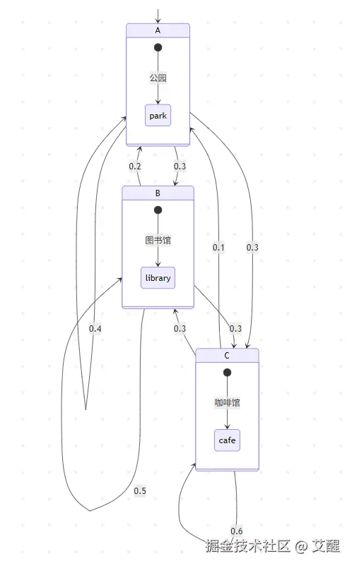
假设你在玩一个简单的游戏，游戏中有三个地点：公园（A）、图书馆（B）和咖啡馆（C）。每天你都会在这三个地点之一度过，并且第二天去的地点只取决于当天所在的地点。

如果你今天在公园（A），明天有 0.4 的概率还在公园，有 0.3 的概率去图书馆，有 0.3 的概率去咖啡馆。
若今天在图书馆（B），明天有 0.2 的概率在公园，有 0.5 的概率还在图书馆，有 0.3 的概率去咖啡馆。
要是今天在咖啡馆（C），明天有 0.1 的概率在公园，有 0.3 的概率在图书馆，有 0.6 的概率还在咖啡馆。

我们可以将这些转移概率整理成转移概率矩阵P：
<math xmlns="http://www.w3.org/1998/Math/MathML" display="block"> P = ( 0.4 0.3 0.3 0.2 0.5 0.3 0.1 0.3 0.6 ) P = \begin{pmatrix} 0.4 & 0.3 & 0.3 \\ 0.2 & 0.5 & 0.3 \\ 0.1 & 0.3 & 0.6 \end{pmatrix} </math>P= 0.40.20.10.30.50.30.30.30.6

公式推导在例子中的应用假设初始时你在公园（即初始状态概率向量 <math xmlns="http://www.w3.org/1998/Math/MathML"> π 0 = [ 1 , 0 , 0 ] \pi_0 = [1, 0, 0] </math>π0=[1,0,0]，我们想知道两天后你在图书馆的概率。根据切普曼 - 柯尔莫哥洛夫方程，两天后的状态概率向量 <math xmlns="http://www.w3.org/1998/Math/MathML"> π 2 \pi_2 </math>π2可以通过 <math xmlns="http://www.w3.org/1998/Math/MathML"> π 2 = π 0 ⋅ P 2 \pi_2 = \pi_0 \cdot P^2 </math>π2=π0⋅P2计算。首先计算 <math xmlns="http://www.w3.org/1998/Math/MathML"> P 2 P^2 </math>P2：
<math xmlns="http://www.w3.org/1998/Math/MathML" display="block"> P 2 = ( 0.4 0.3 0.3 0.2 0.5 0.3 0.1 0.3 0.6 ) ⋅ ( 0.4 0.3 0.3 0.2 0.5 0.3 0.1 0.3 0.6 ) = ( 0.4 × 0.4 + 0.3 × 0.2 + 0.3 × 0.1 0.4 × 0.3 + 0.3 × 0.5 + 0.3 × 0.3 0.4 × 0.3 + 0.3 × 0.3 + 0.3 × 0.6 0.2 × 0.4 + 0.5 × 0.2 + 0.3 × 0.1 0.2 × 0.3 + 0.5 × 0.5 + 0.3 × 0.3 0.2 × 0.3 + 0.5 × 0.3 + 0.3 × 0.6 0.1 × 0.4 + 0.3 × 0.2 + 0.6 × 0.1 0.1 × 0.3 + 0.3 × 0.5 + 0.6 × 0.3 0.1 × 0.3 + 0.3 × 0.3 + 0.6 × 0.6 ) = ( 0.25 0.36 0.39 0.19 0.38 0.43 0.16 0.36 0.48 ) P^2 = \begin{pmatrix} 0.4 & 0.3 & 0.3 \\ 0.2 & 0.5 & 0.3 \\ 0.1 & 0.3 & 0.6 \end{pmatrix} \cdot \begin{pmatrix} 0.4 & 0.3 & 0.3 \\ 0.2 & 0.5 & 0.3 \\ 0.1 & 0.3 & 0.6 \end{pmatrix}\\= \begin{pmatrix} 0.4\times0.4 + 0.3\times0.2 + 0.3\times0.1 & 0.4\times0.3 + 0.3\times0.5 + 0.3\times0.3 & 0.4\times0.3 + 0.3\times0.3 + 0.3\times0.6 \\ 0.2\times0.4 + 0.5\times0.2 + 0.3\times0.1 & 0.2\times0.3 + 0.5\times0.5 + 0.3\times0.3 & 0.2\times0.3 + 0.5\times0.3 + 0.3\times0.6 \\ 0.1\times0.4 + 0.3\times0.2 + 0.6\times0.1 & 0.1\times0.3 + 0.3\times0.5 + 0.6\times0.3 & 0.1\times0.3 + 0.3\times0.3 + 0.6\times0.6 \end{pmatrix}\\= \begin{pmatrix} 0.25 & 0.36 & 0.39 \\ 0.19 & 0.38 & 0.43 \\ 0.16 & 0.36 & 0.48 \end{pmatrix} </math>P2= 0.40.20.10.30.50.30.30.30.6 ⋅ 0.40.20.10.30.50.30.30.30.6 = 0.4×0.4+0.3×0.2+0.3×0.10.2×0.4+0.5×0.2+0.3×0.10.1×0.4+0.3×0.2+0.6×0.10.4×0.3+0.3×0.5+0.3×0.30.2×0.3+0.5×0.5+0.3×0.30.1×0.3+0.3×0.5+0.6×0.30.4×0.3+0.3×0.3+0.3×0.60.2×0.3+0.5×0.3+0.3×0.60.1×0.3+0.3×0.3+0.6×0.6 = 0.250.190.160.360.380.360.390.430.48

然后计算 <math xmlns="http://www.w3.org/1998/Math/MathML"> π 2 \pi_2 </math>π2：
<math xmlns="http://www.w3.org/1998/Math/MathML" display="block"> p i 2 = π 0 ⋅ P 2 = [ 1 , 0 , 0 ] ⋅ ( 0.25 0.36 0.39 0.19 0.38 0.43 0.16 0.36 0.48 ) = [ 0.25 , 0.36 , 0.39 ] pi_2 = \pi_0 \cdot P^2\\= [1, 0, 0] \cdot \begin{pmatrix} 0.25 & 0.36 & 0.39 \\ 0.19 & 0.38 & 0.43 \\ 0.16 & 0.36 & 0.48 \end{pmatrix}\\= [0.25, 0.36, 0.39] </math>pi2=π0⋅P2=[1,0,0]⋅ 0.250.190.160.360.380.360.390.430.48 =[0.25,0.36,0.39]

所以，两天后你在图书馆的概率是 0.36。

例3:网页浏览预测

在互联网中，用户浏览网页的行为可以近似看作一个马尔科夫链。每个网页是一个状态，用户从一个网页跳转到另一个网页的概率构成转移概率矩阵。假设我们有一个包含三个网页（网页 1、网页 2、网页 3）的小型网站。通过分析用户行为数据，得到转移概率矩阵P：
<math xmlns="http://www.w3.org/1998/Math/MathML" display="block"> ( 0.5 0.3 0.2 0.1 0.7 0.2 0.3 0.4 0.3 ) \begin{pmatrix} 0.5 & 0.3 & 0.2 \\ 0.1 & 0.7 & 0.2 \\ 0.3 & 0.4 & 0.3 \end{pmatrix} </math> 0.50.10.30.30.70.40.20.20.3

若初始时用户在网页 1（初始状态概率向量 <math xmlns="http://www.w3.org/1998/Math/MathML"> π 0 = [ 1 , 0 , 0 ] \pi_0 = [1, 0, 0] </math>π0=[1,0,0])，我们想计算 3 次跳转后用户在网页 2 的概率。首先，根据切普曼 - 柯尔莫哥洛夫方程，n步后的状态概率向量 <math xmlns="http://www.w3.org/1998/Math/MathML"> π n = π 0 ⋅ P n \pi_n = \pi_0 \cdot P^n </math>πn=π0⋅Pn。计算 <math xmlns="http://www.w3.org/1998/Math/MathML"> P 3 P^3 </math>P3：

python 复制代码

import numpy as np

P = np.array([
    [0.5, 0.3, 0.2],
    [0.1, 0.7, 0.2],
    [0.3, 0.4, 0.3]
])

P_3 = np.linalg.matrix_power(P, 3)
print(P_3)

通过上述代码计算得到 <math xmlns="http://www.w3.org/1998/Math/MathML"> P 3 P^3 </math>P3后，再计算 <math xmlns="http://www.w3.org/1998/Math/MathML"> π 3 \pi_3 </math>π3：

python 复制代码

pi_0 = np.array([1, 0, 0])
pi_3 = pi_0.dot(P_3)
print(pi_3)

pi_3向量中第二个元素即为 3 次跳转后用户在网页 2 的概率。

例4:天气预测简化模型

假设天气只有晴天、多云、雨天三种状态。通过对历史天气数据的分析，我们得到转移概率矩阵P：
<math xmlns="http://www.w3.org/1998/Math/MathML" display="block"> P = ( 0.7 0.2 0.1 0.3 0.5 0.2 0.2 0.4 0.4 ) P = \begin{pmatrix} 0.7 & 0.2 & 0.1 \\ 0.3 & 0.5 & 0.2 \\ 0.2 & 0.4 & 0.4 \end{pmatrix} </math>P= 0.70.30.20.20.50.40.10.20.4

如果今天是晴天（初始状态概率向量 <math xmlns="http://www.w3.org/1998/Math/MathML"> π 0 = [ 1 , 0 , 0 ] \pi_0 = [1, 0, 0] </math>π0=[1,0,0]），计算 4 天后是雨天的概率。同样，先计算 <math xmlns="http://www.w3.org/1998/Math/MathML"> P 4 P^4 </math>P4：

python 复制代码

P = np.array([
    [0.7, 0.2, 0.1],
    [0.3, 0.5, 0.2],
    [0.2, 0.4, 0.4]
])

P_4 = np.linalg.matrix_power(P, 4)
print(P_4)

然后计算 <math xmlns="http://www.w3.org/1998/Math/MathML"> π 4 \pi_4 </math>π4：

python 复制代码

pi_0 = np.array([1, 0, 0])
pi_4 = pi_0.dot(P_4)
print(pi_4)

pi_4向量中第三个元素就是 4 天后是雨天的概率。虽然实际的天气预测要复杂得多，但马尔科夫链为这种时间序列的状态预测提供了一个简单而有效的基础模型框架。

四、实际应用案例

1. 自然语言处理（NLP）

隐马尔可夫模型（HMM）用于词性标注和语音识别。例如，通过观察单词序列推测隐藏的词性标记。

2. 金融市场分析预测

股票市场的牛市/熊市状态转换。假设转移矩阵为： <math xmlns="http://www.w3.org/1998/Math/MathML"> P = [ 0.9 0.1 0.2 0.8 ] P = \begin{bmatrix}0.9 & 0.1 \\0.2 & 0.8\end{bmatrix} </math>P=[0.90.20.10.8] 表示牛市有90%概率保持，10%概率转熊市；熊市有20%概率转牛市。

3. 蒙特卡洛模拟（MCMC）

Metropolis-Hastings算法通过构建马尔可夫链，对复杂分布进行采样，广泛应用于贝叶斯统计。

总结

从分析诗歌韵律到驱动AlphaGo的决策过程，马尔可夫链展现了数学工具的跨学科魅力。其核心思想------用简单的概率规则描述复杂系统的演化------使其成为人工智能、金融、物理等领域的基础工具。理解马尔可夫链，就是掌握了一把打开随机世界之门的钥匙。