从0开始学习R语言--Day18--分类变量关联性检验

在平时的分析中，关于分类的问题不仅仅会出现在如何将数据分类，还会体现在要如何去挖掘不同分类指甲呢关系，今天我们来学习分类变量关联性检验的相关方法。

卡方检验

通过观察时间中数据的分布来判断原假设是否成立。假设我们是在判断性别和是否吸烟这两个类别的关系，那么我们可以通过调查吸烟的人群中男性和女性的比例，如果两者无关，那么男性和女性的比例应该会差不多，反之则推翻原假设。

Fisher精确检验

就像它的名字一样，当数据量比较小时，我们可以直接去计算事件发生的概率，就像上面那个吸烟的例子一样，假设样本数量只有10，那么我们可以轻松地通过计算知道性别是否和吸烟有关系。

Cramer's V

这个方法，目的是为了在知道是否有关联的前提下，告诉我们这个关联的程度有多高，0代表无关联，0.1-0.3代表弱关联，0.3-0.5代表中等，0.5以上代表强关联。

以下是一个例子：

R 复制代码

# 生成两个分类变量的关联数据（性别 vs 吸烟）
set.seed(123)
n <- 200  # 样本量

# 创建有轻度关联的数据
data <- data.frame(
  gender = sample(c("Male", "Female"), size = n, replace = TRUE, prob = c(0.5, 0.5)),
  smoke = ifelse(runif(n) > 0.6, "Yes", "No")  # 吸烟比例40%
)

# 人为制造关联：男性更可能吸烟
data$smoke[data$gender == "Male"] <- ifelse(
  runif(sum(data$gender == "Male")) > 0.7, "Yes", "No"  # 男性吸烟比例30%
)

# 查看列联表
table(data$gender, data$smoke)

chi_test <- chisq.test(data$gender, data$smoke)
print(chi_test)

# 输出解读：
# p-value < 0.05 表示显著关联
# Pearson's Chi-squared statistic 是卡方值

fisher_test <- fisher.test(data$gender, data$smoke)
print(fisher_test)

# 输出解读：
# p-value 和卡方检验类似，但更适合小样本
install.packages("rcompanion",type = "binary")
library(rcompanion)

# 计算Cramer's V
cramer_v <- cramerV(data$gender, data$smoke)
print(cramer_v)

# 输出示例：
# Cramer V 
# 0.14
# 解释：0.1~0.3表示弱关联

library(ggplot2)

ggplot(data, aes(x = gender, fill = smoke)) +
  geom_bar(position = "dodge") +
  labs(title = "Gender vs Smoking", x = "Gender", y = "Count")

输出：

R 复制代码

         No Yes
  Female 60  43
  Male   70  27
	Pearson's Chi-squared test with Yates' continuity correction

data:  data$gender and data$smoke
X-squared = 3.6607, df = 1, p-value = 0.05571
	Fisher's Exact Test for Count Data

data:  data$gender and data$smoke
p-value = 0.05349
alternative hypothesis: true odds ratio is not equal to 1
95 percent confidence interval:
 0.2843199 1.0126390
sample estimates:
odds ratio 
 0.5398822
Cramer V 
  0.1458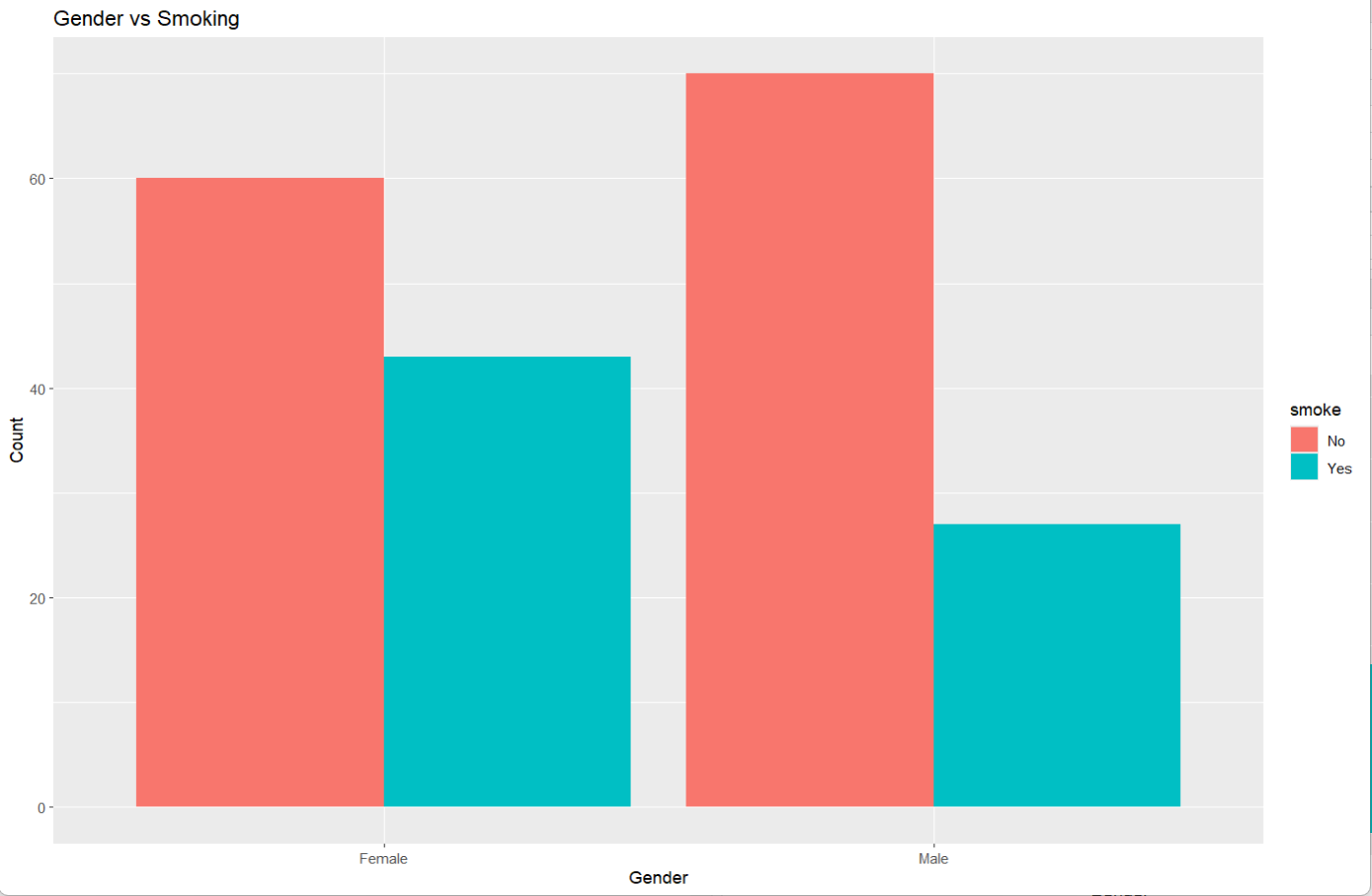

从结果来看，卡方统计量X-squared为3.6607，说明观测值和期望值之间的差异较小；而p大于0.05说明在显著水平下，不能拒绝原假设，即性别和吸烟没有显著联系，但p值在边缘，只比0.05大了一点点，还要仔细验证。fisher检验的p同样大于0.05，只不过它还带来了另一个信息，odds ratio的值为0.5398822，表明男性吸烟的比例比女性低。而Cramer V = 0.1458进一步则进一步说明了吸烟与性别的关联非常弱，三者一起计算，更加确定了这两者无关联的结果的真实性。