Uniswap 流动性机制及相关数学原理分析

摘要

我在研究 Uniswap 白皮书和合约代码时,产生了很多疑问。例如,为什么向池子内添加流动性时必须要保证添加的资产数量维持一个固定的比例?Uniswap V3 中,为什么不同价格区间的流动性,重叠部分可以加在一起进行交易的计算?等等。

这篇文章是我对 Uniswap 有关流动性机制及数学原理的理解和分析,希望能够帮助到 Uniswap 的初学者。文章中,我总结出两条流动性与价格约束规则:

  1. 流动性变化不影响当前资产价格
  2. 资产交易导致价格的变化不影响当前流动性

从这两条规则出发,结合乘积常数方程,就可以推导出 Uniswap 添加流动性、移除流动性、交易资产的公式,我还推导出了流动性叠加原理,解释了为什么一个交易池内只需要维护一个全局流动性变量 <math xmlns="http://www.w3.org/1998/Math/MathML"> L L </math>L 以及在 Uniswap V3 中,为什么不同价格区间的流动性其重叠部分可以加在一起进行计算。

流动性与价格约束规则

我们先从中心化交易所说起,建立一些感性认知。

资产如果进行交易就会有价格,理想状态下这个价格完全由市场,更进一步地说,资产价格应当由买卖双方的需求决定,买入导致价格上涨;卖出导致价格下跌。当然,买卖也可能不会改变资产当前的价格,这取决于下面所说的流动性。

市场里最常见的是拿一种资产换另一种资产的人,称为交易者(Trader 或者 Taker)。另一种人不主动交换资产,而是给交易者行方便,当交易者的对手盘,称为流动性提供者(Liquidity Provider 或者 Maker)或做市商(Market Maker)。

对交易者来说,资产不是想买就有买,想卖就能卖的,这取决于流动性提供者能给他们行多大方便,行的越多,他们买卖起来就越顺畅;行的越少,买卖就受到阻碍。我们把这个方便的程度叫做流动性(Liquidity)。买卖通常涉及两种资产,一种是被交易的资产 X,例如 BTC,称为基础资产,另一种用于标记资产的价格 Y,例如 USDT,称为计价资产。直观感受下,如果流动性提供者提供的资产数量越多,则流动性越大;反之则越少。即流动性 <math xmlns="http://www.w3.org/1998/Math/MathML"> L L </math>L 和资产 X,Y 的数量 <math xmlns="http://www.w3.org/1998/Math/MathML"> x x </math>x, <math xmlns="http://www.w3.org/1998/Math/MathML"> y y </math>y 之间存在某种函数关系 <math xmlns="http://www.w3.org/1998/Math/MathML"> L = f ( x , y ) L = f(x,y) </math>L=f(x,y)。

流动性由流动性提供者提供,他们并没有主动进行买卖操作,前面说过,价格的变化由买卖双方的需求决定,不管流动性提供者向市场中注入更多资产还是减少资产,这都不应该影响当前资产的价格,因此我们引出一条流动性与价格约束性规则:

规则一:流动性变化不影响当前资产价格。

交易者如果买入或者卖出资产,实际上就是跟流动性提供者进行交易,将他们手里的一种资产 X 换成另一种资产 Y。乍一看,流动性提供者手里的资产 Y 减少了,这对以后想买 Y 资产的交易者来说,他的方便程度就没那么大了,或者说 Y 资产的流动性减少了。但是别忘了,流动性手里 X 的资产却增多了,这就更加方便了想买 X 资产的人,也可以说 X 资产的流动性增加了。交易导致价格变化,但资产仅是由一种形式转为另一种形式,流动性提供者提供的流动性不应该变化,因此我们引出另一条流动性与价格约束性规则:

规则二:资产交易导致价格的变化不影响当前流动性

另外我们还注意到,交易者将资产 X 换成 Y,对应地,流动性提供者手里的资产 Y 则变成了 X,其后果就如同交易者和流动性提供者交换了两种资产,因此这种行为也叫做交换资产(Swap)。

以上所述的两条关于流动性与价格约束性规则,在 Uniswap 世界里就是铁律,这也是帮助我们理解 Uniswap 背后的机理以及各种数学公式的基础。接下来我们将从这两条原理出发,一步步推导出 Uniswap 添加流动性、移除流动性、交换资产的所有数学公式,相信能够帮助初学者彻底搞明白看白皮书和合约代码时的困惑。

另外虽然 Uniswap V3 看似机制复杂了很多,但实际上背后的原理仍与 V2 一模一样,所以我会将 V2 和 V3 混在一起进行分析。

乘积常数与流动性

Uniswap 将资产 X 和 Y 组成的交易对叫做一个池子,池子里存储了资产 X 和资产 Y。设资产 X 的储量(Reserve,亦即数量)为 <math xmlns="http://www.w3.org/1998/Math/MathML"> x x </math>x,资产 Y 的储量为 <math xmlns="http://www.w3.org/1998/Math/MathML"> y y </math>y,Uniswap V2 中将资产储量的比值定义为资产的价格(Price),将储量的乘积的平方根定义为流动性(Liquidity),写成数学公式就是:

P_x = \frac{y}{x} = P \tag{1}

P_y = \frac{x}{y} = \frac{1}{P} \tag{2}

L = f(x,y) = \sqrt{xy} \tag{3}

或者:

L^2 = xy = k \tag{4}

其中 <math xmlns="http://www.w3.org/1998/Math/MathML"> P x P_x </math>Px, <math xmlns="http://www.w3.org/1998/Math/MathML"> P y P_y </math>Py 分别为资产 X 和 Y 的价格, <math xmlns="http://www.w3.org/1998/Math/MathML"> k k </math>k 称为乘积常数,其平方根 <math xmlns="http://www.w3.org/1998/Math/MathML"> L L </math>L 称为流动性。资产价格 <math xmlns="http://www.w3.org/1998/Math/MathML"> P x P_x </math>Px, <math xmlns="http://www.w3.org/1998/Math/MathML"> P y P_y </math>Py 之间的关系互为倒数,因此只需要关注其中一个值即可,一般我们习惯将 X 作为基础资产(例如 BTC),将 Y 作为计价资产(例如 USDT),因此后续提及价格 <math xmlns="http://www.w3.org/1998/Math/MathML"> P P </math>P 指的是公式 (1) 定义的价格。

根据规则一,添加或移除流动性导致 <math xmlns="http://www.w3.org/1998/Math/MathML"> L L </math>L 增加或减少(对应的就是储量 <math xmlns="http://www.w3.org/1998/Math/MathML"> x x </math>x 和 <math xmlns="http://www.w3.org/1998/Math/MathML"> y y </math>y 增加或减少),价格 <math xmlns="http://www.w3.org/1998/Math/MathML"> P x P_x </math>Px 和 <math xmlns="http://www.w3.org/1998/Math/MathML"> P y P_y </math>Py 不变。根据规则二,交易导致储量 <math xmlns="http://www.w3.org/1998/Math/MathML"> x x </math>x, <math xmlns="http://www.w3.org/1998/Math/MathML"> y y </math>y 一方增加一方减少,价格 <math xmlns="http://www.w3.org/1998/Math/MathML"> P P </math>P 发生变化,但 <math xmlns="http://www.w3.org/1998/Math/MathML"> L L </math>L 始终为常数。

这里你可能会有一个疑惑,公式 (1) 或者 (2) 中,我只要调整 <math xmlns="http://www.w3.org/1998/Math/MathML"> y y </math>y 和 <math xmlns="http://www.w3.org/1998/Math/MathML"> x x </math>x 的比例,比如单纯地增大 <math xmlns="http://www.w3.org/1998/Math/MathML"> y y </math>y,不就使得价格升高且流动性增加,从而跟上述两个规则冲突了吗?但事实并非如此。

我们说了规则在 Uniswap 的世界里就是铁律,既然铁律就不能违背,那就只能认为单纯增加的 <math xmlns="http://www.w3.org/1998/Math/MathML"> y y </math>y 没有任何作用,它不参与任何流动性和 交易有关的计算,增加的量就像进了黑洞。

公式 (4) 画成函数图像就是下面这个样子:
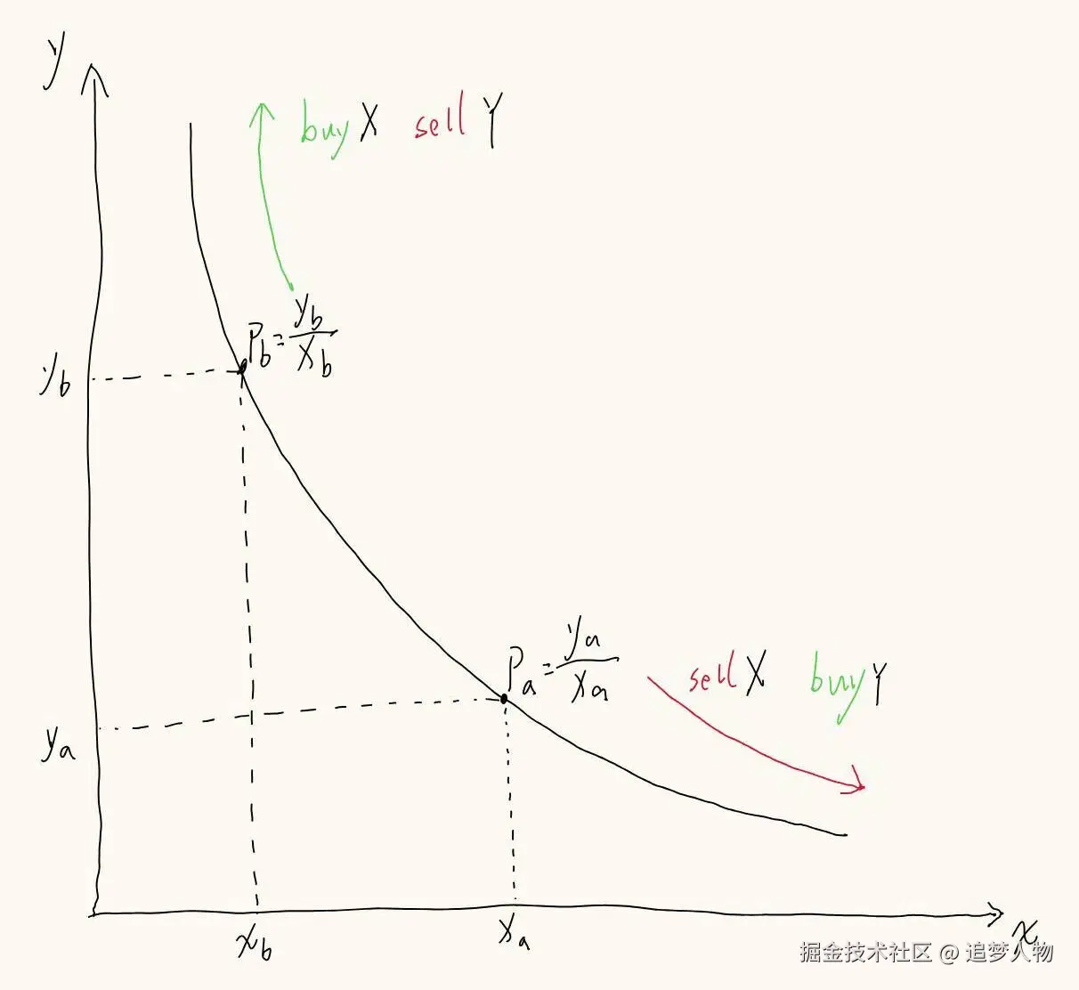

图 1:乘积常数函数 <math xmlns="http://www.w3.org/1998/Math/MathML"> x y = k xy=k </math>xy=k 的图像。点 a 的坐标为 <math xmlns="http://www.w3.org/1998/Math/MathML"> ( y a , x a ) (y_a,x_a) </math>(ya,xa),对应资产价格 <math xmlns="http://www.w3.org/1998/Math/MathML"> P a = y a x a P_a=\frac{y_a}{x_a} </math>Pa=xaya;点 b 的坐标为 <math xmlns="http://www.w3.org/1998/Math/MathML"> ( y b , x b ) (y_b,x_b) </math>(yb,xb),对应资产价格 <math xmlns="http://www.w3.org/1998/Math/MathML"> P b = y b x b P_b=\frac{y_b}{x_b} </math>Pb=xbyb。价格 <math xmlns="http://www.w3.org/1998/Math/MathML"> P P </math>P 只能沿着曲线变动,越往右下, <math xmlns="http://www.w3.org/1998/Math/MathML"> x x </math>x 越多而 <math xmlns="http://www.w3.org/1998/Math/MathML"> y y </math>y 越少,说明交易方向是卖出 X 买入 Y,X 的价格 <math xmlns="http://www.w3.org/1998/Math/MathML"> P P </math>P 越来越低;越往左上, <math xmlns="http://www.w3.org/1998/Math/MathML"> x x </math>x 越少而 <math xmlns="http://www.w3.org/1998/Math/MathML"> y y </math>y 越多,说明交易方向是买入 X 卖出 Y,X 的价格 <math xmlns="http://www.w3.org/1998/Math/MathML"> P P </math>P 越来越高。

以上就是 Uniswap V2 的核心。但是仔细观察函数图像我们会发现一些不太完美的地方,价格 <math xmlns="http://www.w3.org/1998/Math/MathML"> P P </math>P 可以趋近于 0 和无穷大,这种情况理论上是存在的,但现实中很少见。现实中资产价格总在特定范围内波动,于是我们对这条曲线进行改进,引入限价范围,流动性集中在此范围内,超出此价格范围若无流动性提供,则无法进行交易。如此改进后,我们就来到了 Uniswap V3。

为了理解 V3 是如何优化的,我们先不做任何其他操作,只单纯在 V2 的曲线上引入一个限价范围,假设就限定价格在 <math xmlns="http://www.w3.org/1998/Math/MathML"> P a P_a </math>Pa 和 <math xmlns="http://www.w3.org/1998/Math/MathML"> P b P_b </math>Pb 之间,规定价格触及 <math xmlns="http://www.w3.org/1998/Math/MathML"> P a P_a </math>Pa 后,无法再往更高的价格推进,也就是不再允许买 X 卖 Y 了(但注意反向交易会把价格拉回区间,这是可以的);价格触及 <math xmlns="http://www.w3.org/1998/Math/MathML"> P b P_b </math>Pb 后,无法再往更低的价格推进,也就是不再允许卖 X 买 Y 了。这个机制有点类似于中国 A 股的涨跌停限制。

但是这样规定后仍然存在一个问题,就是价格触及边界后,实际上池子里的 X 和 Y 资产仍有储量,交易理论上是可以继续向边界外的价格推进的,只是我们人为卡死了。

既然限价范围外无法再交易,多余的资产储量已经没有意义,因此我们希望当价格触达边界时,不允许再被买入的那一方资产数量变为 0,同时交易仍然遵规则二,那么我们就得到了图中蓝色曲线:


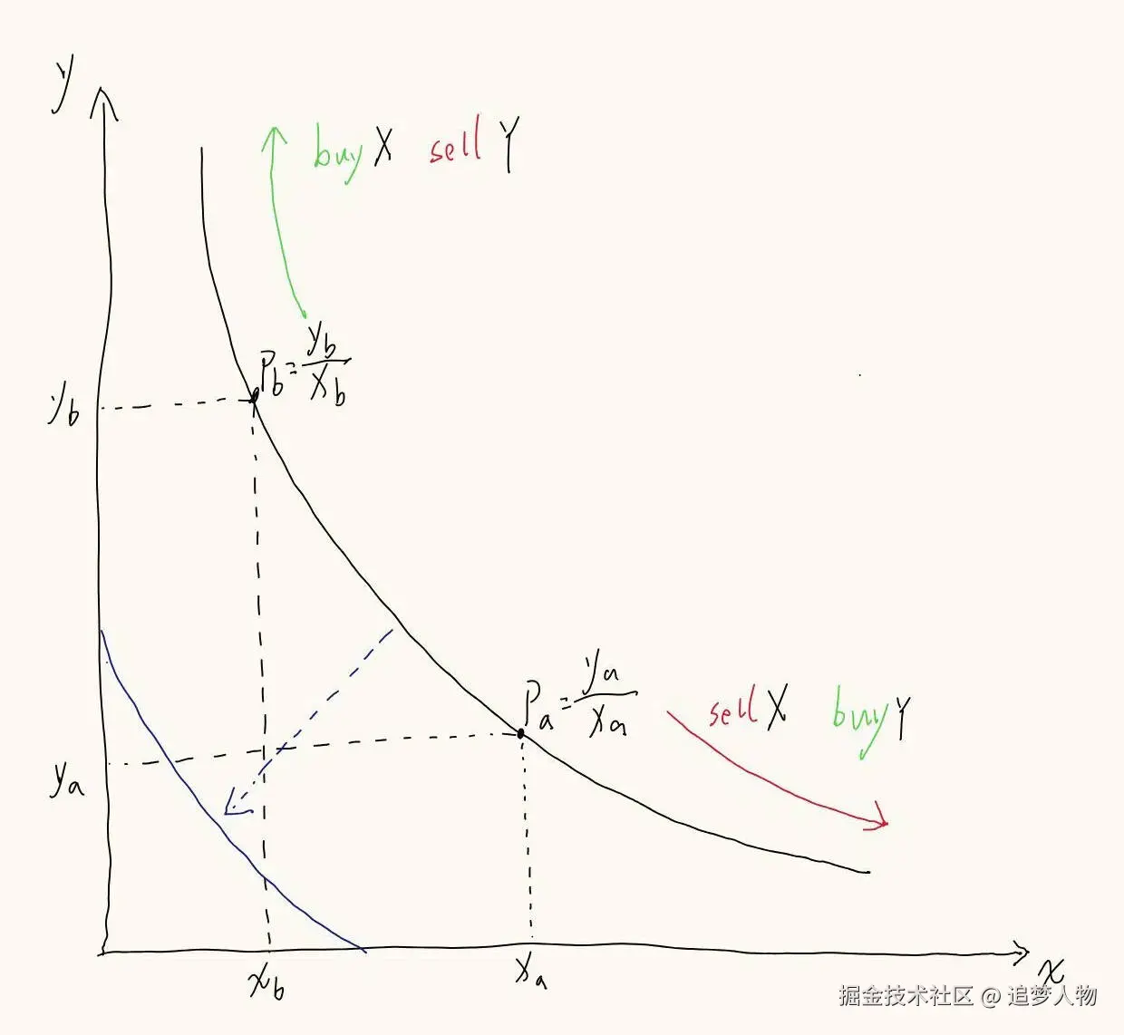
图 2:限价范围内的乘积常数函数图像,其与 x 轴和 y 轴的交点表示价格边界,可以看到在价格边界处,某一方的资产储量等于 0。曲线上任意一点的坐标值相乘仍为常数。

我们把 V2 的曲线也画在了坐标系内,是为了方便地观察到,蓝色曲线实际就是 V2 曲线向下平移 <math xmlns="http://www.w3.org/1998/Math/MathML"> y a y_a </math>ya 再向左平移 <math xmlns="http://www.w3.org/1998/Math/MathML"> x b x_b </math>xb 得到的,所以我们可以写出其曲线方程为:

(x+x_b)(y+y_a)=L^2 \tag{5}

和 Uniswap V2 不同,V3 不跟踪资产的储量,而是跟踪价格 <math xmlns="http://www.w3.org/1998/Math/MathML"> P P </math>P 和流动性 <math xmlns="http://www.w3.org/1998/Math/MathML"> L L </math>L,因此我们对公式 (5) 稍作变换,将常量 <math xmlns="http://www.w3.org/1998/Math/MathML"> x b x_b </math>xb 和 <math xmlns="http://www.w3.org/1998/Math/MathML"> y a y_a </math>ya 表示为 <math xmlns="http://www.w3.org/1998/Math/MathML"> P P </math>P 跟 <math xmlns="http://www.w3.org/1998/Math/MathML"> L L </math>L 的关系式。

点 <math xmlns="http://www.w3.org/1998/Math/MathML"> a a </math>a 和 <math xmlns="http://www.w3.org/1998/Math/MathML"> b b </math>b 是公式 (4) 定义的曲线上的点,因此其满足:

\frac{y_a}{x_a}=P_a \tag{6}

x_ay_a=L^2 \tag{7}

\frac{y_b}{x_b}=P_b \tag{8}

x_by_b=L^2 \tag{9}

公式 (7) 两边同时除以 <math xmlns="http://www.w3.org/1998/Math/MathML"> y a 2 y_a^2 </math>ya2 再结合公式 (6),得 <math xmlns="http://www.w3.org/1998/Math/MathML"> x a y a = L 2 y a 2 = 1 P a \frac{x_a}{y_a} = \frac{L^2}{y_a^2} = \frac{1}{P_a} </math>yaxa=ya2L2=Pa1,解得 <math xmlns="http://www.w3.org/1998/Math/MathML"> y a = L P a y_a = L\sqrt{P_a} </math>ya=LPa 同理,公式 (9) 两边同时除以 <math xmlns="http://www.w3.org/1998/Math/MathML"> x b 2 x_b^2 </math>xb2 再结合公式 (8),得 <math xmlns="http://www.w3.org/1998/Math/MathML"> y b x b = L 2 x b 2 = P b \frac{y_b}{x_b} = \frac{L^2}{x_b^2} = P_b </math>xbyb=xb2L2=Pb,解得 <math xmlns="http://www.w3.org/1998/Math/MathML"> x b = L P b x_b = \frac{L}{\sqrt{P_b}} </math>xb=Pb L

代入公式 (5),得到限价范围内的乘积常数函数方程:

(x+\frac{L}{\sqrt{P_b}})(y+L\sqrt{P_a})=L^2 \tag{10}

我们把 <math xmlns="http://www.w3.org/1998/Math/MathML"> L P b \frac{L}{\sqrt{P_b}} </math>Pb L 和 <math xmlns="http://www.w3.org/1998/Math/MathML"> L P a L\sqrt{P_a} </math>LPa 叫做虚拟储量, <math xmlns="http://www.w3.org/1998/Math/MathML"> x x </math>x, <math xmlns="http://www.w3.org/1998/Math/MathML"> y y </math>y 是实际储量。需要注意的是,价格不是实际储量的比值 <math xmlns="http://www.w3.org/1998/Math/MathML"> y / x y/x </math>y/x,而是加上虚拟储量后的比值。Uniswap V3 中直接跟踪价格 <math xmlns="http://www.w3.org/1998/Math/MathML"> P P </math>P,所以大部分情况下不需要关心虚拟储量的具体值。可以把虚拟储量理解为 V2 曲线到达价格边界时,无法再被买入那一方资产的剩余储量,因为价格被限制了,无法再往相同方向继续推进,所以这个剩余的储量并不需要实际提供,在系统中给一个虚拟值参与计算即可。

在价格边界处只剩一种资产,接下来我们来推导该资产实际储量的表达式。在 <math xmlns="http://www.w3.org/1998/Math/MathML"> a a </math>a 处,资产 Y 的储量为 0,代入公式 (10) 得:

<math xmlns="http://www.w3.org/1998/Math/MathML"> ( x + L P b ) ( 0 + L P a ) = L 2 (x+\frac{L}{\sqrt{P_b}})(0+L\sqrt{P_a})=L^2 </math>(x+Pb L)(0+LPa )=L2

解得:

x = \frac{L}{\sqrt{P_a}} - \frac{L}{\sqrt{P_b}} = L\frac{\sqrt{P_b} - \sqrt{P_a}}{\sqrt{P_a}\sqrt{P_b}} \tag{11}

同理可求得点 <math xmlns="http://www.w3.org/1998/Math/MathML"> b b </math>b 处资产 Y 的储量:

y = L(\sqrt{P_b} - \sqrt{P_a}) \tag{12}

当价格 <math xmlns="http://www.w3.org/1998/Math/MathML"> P P </math>P 处于 <math xmlns="http://www.w3.org/1998/Math/MathML"> P a P_a </math>Pa 和 <math xmlns="http://www.w3.org/1998/Math/MathML"> P b P_b </math>Pb 内,我们知道价格 <math xmlns="http://www.w3.org/1998/Math/MathML"> P P </math>P 的表达式:

P = \frac{y+L\sqrt{P_a}}{x+\frac{L}{\sqrt{P_b}}} \tag{13}

移项得到:

<math xmlns="http://www.w3.org/1998/Math/MathML"> y = P ( x + L P b ) − L P a y = P(x+\frac{L}{\sqrt{P_b}}) - L\sqrt{P_a} </math>y=P(x+Pb L)−LPa

将其代入公式 (10):

<math xmlns="http://www.w3.org/1998/Math/MathML"> ( x + L P b ) ( P ( x + L P b ) − L P a + L P a ) = L 2 (x+\frac{L}{\sqrt{P_b}})(P(x+\frac{L}{\sqrt{P_b}}) - L\sqrt{P_a}+L\sqrt{P_a})=L^2 </math>(x+Pb L)(P(x+Pb L)−LPa +LPa )=L2

解得:

x = \frac{L}{\sqrt{P}} - \frac{L}{\sqrt{P_b}} = L\frac{\sqrt{P_b} - \sqrt{P}}{\sqrt{P}\sqrt{P_b}} \tag{14}

同理可求的:

y = L(\sqrt{P} - \sqrt{P_a}) \tag{15}

总结起来就是,池子价格 <math xmlns="http://www.w3.org/1998/Math/MathML"> P P </math>P,流动性 <math xmlns="http://www.w3.org/1998/Math/MathML"> L L </math>L 以及边界价格 <math xmlns="http://www.w3.org/1998/Math/MathML"> P a P_a </math>Pa 和 <math xmlns="http://www.w3.org/1998/Math/MathML"> P b P_b </math>Pb,资产 X 和 Y 的真实储量 <math xmlns="http://www.w3.org/1998/Math/MathML"> x x </math>x 和 <math xmlns="http://www.w3.org/1998/Math/MathML"> y y </math>y 直接的约束关系由公式 (11) (12) (14) (15) 给出。这几个约束关系非常重要,在 Uniswap V3 的实际应用中,我们通常已知边界价格 <math xmlns="http://www.w3.org/1998/Math/MathML"> P a P_a </math>Pa 和 <math xmlns="http://www.w3.org/1998/Math/MathML"> P b P_b </math>Pb,当前价格 <math xmlns="http://www.w3.org/1998/Math/MathML"> P P </math>P,以及其中某个资产的真实储量,需要计算另一个资产所需的真实储量和流动性 <math xmlns="http://www.w3.org/1998/Math/MathML"> L L </math>L。

对公式 (14) (15) 稍加变形,我们得到两个流动性公式计算公式:

L = x\frac{\sqrt{P}\sqrt{P_b}}{\sqrt{P_b} - \sqrt{P}} = \frac{y}{\sqrt{P} - \sqrt{P_a}} \tag{16}

乍一看好像流动性只由其中一种资产的真实储量 <math xmlns="http://www.w3.org/1998/Math/MathML"> x x </math>x 或者 <math xmlns="http://www.w3.org/1998/Math/MathML"> y y </math>y 及当前价格 <math xmlns="http://www.w3.org/1998/Math/MathML"> P P </math>P 决定,但实际上不是。注意式中的变量 <math xmlns="http://www.w3.org/1998/Math/MathML"> P P </math>P,资产 X 和 Y 的储量共同决定了价格,因此实际上流动性依然由 X 和 Y 的储量共同决定,只是公式中将单个资产的储量隐藏了。

改变流动性

改变流动性的操作包括添加流动性和移除流动性。添加流动性即增加资产 X 和 Y 的储量,移除流动性即减少储量。

我们先来分析添加流动性需要遵循的约束条件。

先来推导 Uniswap V2 中添加流动性的公式,添加流动性时有两种情况:一是池子还不存在,也就是说资产 X 和 Y 还没有任何储量,都是 0,Uniswap 中这种情况下添加流动性也叫做初始化池子;二是资产 X 和 Y 已有储量的情况下再向池子里添加更多的储量。

先来看情况一,这种情况比较简单,根据流动性变化不影响当前资产价格的规则(规则一),添加流动性不能改变资产当前价格,但价格由储量的比值定义,此时没有储量,也就是价格未定义。这种情况下,通常参考其他市场的价格作为当前资产价格,只需保证增加的资产储量比值等于这个价格就行。

值得注意的是,Uniswap 并不限制流动性提供者一定要按照参考价格的比例添加资产储量,但是如果不按比例添加,Uniswap 中的资产价格与外部市场价格就会有差异,这会导致套利,套利导致的后果对流动性提供者不利,所以理性的流动性提供者一定会按照参考价格严格控制初始储量的比例。

再来看情况二,此时资产 X 和 Y 已有储量 <math xmlns="http://www.w3.org/1998/Math/MathML"> x x </math>x, <math xmlns="http://www.w3.org/1998/Math/MathML"> y y </math>y,假设资产 X,Y 增加的储量分别为 <math xmlns="http://www.w3.org/1998/Math/MathML"> Δ x \Delta{x} </math>Δx 和 <math xmlns="http://www.w3.org/1998/Math/MathML"> Δ y \Delta{y} </math>Δy,根据规则一,资产价格在添加流动性前后不变,也就是:

\frac{y}{x} = \frac{y + \Delta{y}}{x + \Delta{x}} \tag{17}

联立公式 (17) 和 (1),稍加变形我们解得下面的关系式子:

\frac{\Delta{y}}{\Delta{x}} = \frac{y}{x} = P \tag{18}

公式 (18) 说明,当资产已有储量,添加流动性时,提供的两种资产的量必须成比例,且比值就是当前价格。根据这个约束关系式即确定 <math xmlns="http://www.w3.org/1998/Math/MathML"> Δ x \Delta{x} </math>Δx 和 <math xmlns="http://www.w3.org/1998/Math/MathML"> Δ y \Delta{y} </math>Δy 的数量,既然两者数量已确定,那么其乘积为常数,设:

\Delta{x}\Delta{y} = d^2 \tag{19}

联立公式 (18) 和 (19),我们可以写出:

d = \Delta{x}\sqrt{P} = \Delta{x}\sqrt{\frac{y}{x}} = \Delta{x}\sqrt{\frac{xy}{xx}} = L\frac{\Delta{x}}{x} \tag{20}

同理可得:

d = \frac{\Delta{y}}{\sqrt{P}} = \frac{\Delta{y}}{\sqrt{\frac{y}{x}}} = \frac{\Delta{y}}{\sqrt{\frac{yy}{xy}}} = L\frac{\Delta{y}}{y} \tag{21}

公式 (20) (21) 可以让我们看出一些端倪,如果我们将 <math xmlns="http://www.w3.org/1998/Math/MathML"> d d </math>d 定义为流动性增量,将符号重新写成 <math xmlns="http://www.w3.org/1998/Math/MathML"> Δ L \Delta{L} </math>ΔL,上面的式子说明,流动性提供者向池子中添加了储量 <math xmlns="http://www.w3.org/1998/Math/MathML"> Δ x \Delta{x} </math>Δx 和 <math xmlns="http://www.w3.org/1998/Math/MathML"> Δ y \Delta{y} </math>Δy,这两个储量贡献了流动性 <math xmlns="http://www.w3.org/1998/Math/MathML"> Δ L \Delta{L} </math>ΔL。在 Uniswap V2 中,系统会将贡献的流动性铸成流动性代币(Liquidity Token)给流动性提供者,流动性代币的数量由公式 (20) 和 (21) 给出。这个流动性代币的作用就是记录流动性提供者贡献的流动性,因为在移除流动性时需要根据这个数来计算返还给流动性提供者的资产 X 和 Y 的数量。实际上,我们的目的是记录下每个流动性提供者贡献的流动性 <math xmlns="http://www.w3.org/1998/Math/MathML"> Δ L \Delta{L} </math>ΔL,记录的方式并不重要。Uniswap V2 中是通过铸造流动性代币的方式记录,但我个人觉得有点多次一举,到了 V3 就不再铸造流动性代币了,而是直接把 <math xmlns="http://www.w3.org/1998/Math/MathML"> Δ L \Delta{L} </math>ΔL 记到智能合约的某个变量里。

上面讨论的内容假设了 <math xmlns="http://www.w3.org/1998/Math/MathML"> Δ x \Delta{x} </math>Δx 和 <math xmlns="http://www.w3.org/1998/Math/MathML"> Δ y \Delta{y} </math>Δy 都大于 0,若 <math xmlns="http://www.w3.org/1998/Math/MathML"> Δ x \Delta{x} </math>Δx 和 <math xmlns="http://www.w3.org/1998/Math/MathML"> Δ y \Delta{y} </math>Δy 都小于 0,表明流动性提供者正在移除流动性,根据规则一,容易推导出上述公式仍然成立。此时流动性提供者返还添加流动性时铸造的流动性代币数量 <math xmlns="http://www.w3.org/1998/Math/MathML"> Δ L \Delta{L} </math>ΔL,获得的资产 X 和 Y 的数量由下式给出:

\Delta{x} = \frac{\Delta{L}}{L}x \tag{22}

\Delta{y} = \frac{\Delta{L}}{L}y \tag{23}

值得注意的是,这个式子中的 <math xmlns="http://www.w3.org/1998/Math/MathML"> x x </math>x, <math xmlns="http://www.w3.org/1998/Math/MathML"> y y </math>y 和 <math xmlns="http://www.w3.org/1998/Math/MathML"> L L </math>L 是移除流动性时资产 X,Y 的储量以及总的流动性,而不是流动性提供者添加流动性时的值。

很多分析 Uniswap 的文章在提及添加和移除流动性时,一般都是说为了维护池子的平衡,需要按照一定的比例添加或者移除资产,但为什么一定要按比例来并未明说,这给研究 Uniswap 实现原理的新人带来很大困惑(至少对我来说是这样)。以上推导过程解释了为什么要这样做,本质上是由于规则二的约束。

上面式子还说明了,只要价格发生了变化(即储量比例发生了变化),移除流动性时获得的资产量 <math xmlns="http://www.w3.org/1998/Math/MathML"> Δ x \Delta{x} </math>Δx 和 <math xmlns="http://www.w3.org/1998/Math/MathML"> Δ y \Delta{y} </math>Δy 与添加流动性时提供的资产量 <math xmlns="http://www.w3.org/1998/Math/MathML"> Δ x \Delta{x} </math>Δx 和 <math xmlns="http://www.w3.org/1998/Math/MathML"> Δ y \Delta{y} </math>Δy 就不是同一个值,这也就是导致无常损失的原因。之所以称为损失,是因为可以证明移除流动性获得的资产价值一定不高于添加流动性时资产的价值。从上述公式不难推导出无常损失的代数表达式,感兴趣的同学可以自行证明。

还有一点值得注意,假设 <math xmlns="http://www.w3.org/1998/Math/MathML"> x y = L 2 xy = L^2 </math>xy=L2 是第一个流动性提供者添加的流动性,第二个流动性提供者继续添加 <math xmlns="http://www.w3.org/1998/Math/MathML"> Δ x \Delta{x} </math>Δx 和 <math xmlns="http://www.w3.org/1998/Math/MathML"> Δ y \Delta{y} </math>Δy,使得流动性变为 <math xmlns="http://www.w3.org/1998/Math/MathML"> L + Δ L L + \Delta{L} </math>L+ΔL,这就像是一个流动性为 <math xmlns="http://www.w3.org/1998/Math/MathML"> L L </math>L 的池子和一个流动性为 <math xmlns="http://www.w3.org/1998/Math/MathML"> Δ L \Delta{L} </math>ΔL 的池子叠加在了一起,第一个流动性提供者贡献流动性 <math xmlns="http://www.w3.org/1998/Math/MathML"> L L </math>L,第二个贡献流动性 <math xmlns="http://www.w3.org/1998/Math/MathML"> Δ L \Delta{L} </math>ΔL。这个性质对于后续我们说明流动性叠加原理时非常重要。

接下来我们开始推导 Uniswap V3 添加流动的公式。思路是一样的,只是公式更加复杂,需要一些耐心。

前面提到过,Uniswap V3 资产储备和流动性的约束关系有公式 (10) 给出:

<math xmlns="http://www.w3.org/1998/Math/MathML"> ( x + L P b ) ( y + L P a ) = L 2 (x+\frac{L}{\sqrt{P_b}})(y+L\sqrt{P_a})=L^2 </math>(x+Pb L)(y+LPa )=L2

和 V2 一样,第一次添加流动性时价格未定义,通常参考一个外部市场的价格,使得添加的储量(真实+虚拟储量)的比例等于这个价格,且满足上面的关系式子。实际操作中,我们首先确定一种资产需添加的量,例如 <math xmlns="http://www.w3.org/1998/Math/MathML"> x x </math>x,如果参考的价格在指定的限价范围之内,则根据公式 (16) 算出 <math xmlns="http://www.w3.org/1998/Math/MathML"> L L </math>L,再根据公式 (15) 算出 <math xmlns="http://www.w3.org/1998/Math/MathML"> y y </math>y。如果在限价范围外,则根据当前价格应用公式 (11) 或者 (12)。

假设资产 X 和 Y 已有储量,这时候添加 <math xmlns="http://www.w3.org/1998/Math/MathML"> Δ x \Delta{x} </math>Δx 和 <math xmlns="http://www.w3.org/1998/Math/MathML"> Δ y \Delta{y} </math>Δy 应该满足什么关系式呢?为了简单起见,我们假设当前价格 <math xmlns="http://www.w3.org/1998/Math/MathML"> P P </math>P 处于限价范围内(限价范围外的结论一致,可自行推导),仍然根据规则二,我们有:

\frac{y+L\sqrt{P_a}}{x+\frac{L}{\sqrt{P_b}}} = \frac{y+\Delta{y}+L'\sqrt{P_a}}{x+\Delta{x}+\frac{L'}{\sqrt{P_b}}} = P \tag{24}

需要注意的是,当 <math xmlns="http://www.w3.org/1998/Math/MathML"> Δ x \Delta{x} </math>Δx 和 <math xmlns="http://www.w3.org/1998/Math/MathML"> Δ y \Delta{y} </math>Δy 添加后,总的流动性不再是添加之前的 <math xmlns="http://www.w3.org/1998/Math/MathML"> L L </math>L,而是变成新的值 <math xmlns="http://www.w3.org/1998/Math/MathML"> L ′ L' </math>L′,所以连等式中间项流动性用的是 <math xmlns="http://www.w3.org/1998/Math/MathML"> L ′ L' </math>L′。设流动性的改变量为 <math xmlns="http://www.w3.org/1998/Math/MathML"> Δ L \Delta{L} </math>ΔL,即 <math xmlns="http://www.w3.org/1998/Math/MathML"> L ′ − L = Δ L L' - L = \Delta{L} </math>L′−L=ΔL,代入上式,得到:

\frac{y+L\sqrt{P_a}}{x+\frac{L}{\sqrt{P_b}}} = \frac{y+\Delta{y}+(L+\Delta{L})\sqrt{P_a}}{x+\Delta{x}+\frac{L+\Delta{L}}{\sqrt{P_b}}} = P \tag{25}

将连等式左边两项做一些移项、消除同项等操作,虽然很繁琐,但最终我们可以得到:

x\Delta{y} + \Delta{y}\frac{L}{\sqrt{P_b}} + \Delta{L}\sqrt{P_a}x = y\Delta{x} + \Delta{x}L\sqrt{P_a} + \frac{\Delta{L}}{\sqrt{P_b}}y \tag{26}

公式 (14) 和 (15) 给出了 <math xmlns="http://www.w3.org/1998/Math/MathML"> x x </math>x 和 <math xmlns="http://www.w3.org/1998/Math/MathML"> y y </math>y 的表达式,代入上式并化简,最终我们可以得到:

\frac{\Delta{y} + \Delta{L}\sqrt{P_a}}{\Delta{x}+\frac{\Delta{L}}{\sqrt{P_b}}} = P = \frac{y+L\sqrt{P_a}}{x+\frac{L}{\sqrt{P_b}}} \tag{27}

可以发现,这个式子和定义价格的公式 (13) 形式上完全一样。这就是 <math xmlns="http://www.w3.org/1998/Math/MathML"> Δ x \Delta{x} </math>Δx 和 <math xmlns="http://www.w3.org/1998/Math/MathML"> Δ y \Delta{y} </math>Δy 需满足的式子,也就是说,当向池子中添加流动性时,添加的资产量 <math xmlns="http://www.w3.org/1998/Math/MathML"> Δ x \Delta{x} </math>Δx 和 <math xmlns="http://www.w3.org/1998/Math/MathML"> Δ y \Delta{y} </math>Δy 使得流动性增加 <math xmlns="http://www.w3.org/1998/Math/MathML"> Δ L \Delta{L} </math>ΔL,其必须满足上面的式子。

但是上面的式子不太容易解出 <math xmlns="http://www.w3.org/1998/Math/MathML"> Δ x \Delta{x} </math>Δx 和 <math xmlns="http://www.w3.org/1998/Math/MathML"> Δ y \Delta{y} </math>Δy。类似于 V2 中的处理方式, <math xmlns="http://www.w3.org/1998/Math/MathML"> Δ x \Delta{x} </math>Δx 和 <math xmlns="http://www.w3.org/1998/Math/MathML"> Δ y \Delta{y} </math>Δy 确定之后, <math xmlns="http://www.w3.org/1998/Math/MathML"> Δ L \Delta{L} </math>ΔL 随之确定,以下式子为常数并令其等于 <math xmlns="http://www.w3.org/1998/Math/MathML"> d 2 d^2 </math>d2:

(\Delta{x} + \frac{\Delta{L}}{\sqrt{P_b}})(\Delta{y} + \Delta{L}\sqrt{P_a}) = d^2 \tag{28}

结合公式 (27),和 V2 中的处理方式一样,我们有:

d = (\Delta{x} + \frac{\Delta{L}}{\sqrt{P_b}})\sqrt{P} = (\Delta{x} + \frac{\Delta{L}}{\sqrt{P_b}})\sqrt{\frac{y+L\sqrt{P_a}}{x + \frac{L}{\sqrt{P_b}}}} = (\Delta{x} + \frac{\Delta{L}}{\sqrt{P_b}})\sqrt{\frac{L^2}{(x + \frac{L}{\sqrt{P_b}})^2}} = L\frac{\Delta{x} + \frac{\Delta{L}}{\sqrt{P_b}}}{x + \frac{L}{\sqrt{P_b}}} \tag{29}

同理可得:

d = L\frac{\Delta{y} + \Delta{L}\sqrt{P_a}}{y + L\sqrt{P_a}} \tag{30}

两式相乘,我们得到:

d^2 = (\Delta{x} + \frac{\Delta{L}}{\sqrt{P_b}})(\Delta{y} + \Delta{L}\sqrt{P_a}) \tag{31}

可以发现公式 (31) 的形式和公式 (10) 非常接近,这不禁让我们猜测, <math xmlns="http://www.w3.org/1998/Math/MathML"> d d </math>d 是否等于 <math xmlns="http://www.w3.org/1998/Math/MathML"> Δ L \Delta{L} </math>ΔL 呢?事实上是的。我们考察价格处于边界时的情况,假设价格处于点 <math xmlns="http://www.w3.org/1998/Math/MathML"> b b </math>b,价格 <math xmlns="http://www.w3.org/1998/Math/MathML"> P = P b P = P_b </math>P=Pb,在该点处只需要 <math xmlns="http://www.w3.org/1998/Math/MathML"> Δ y \Delta{y} </math>Δy, <math xmlns="http://www.w3.org/1998/Math/MathML"> Δ x = 0 \Delta{x} = 0 </math>Δx=0,代入公式 (27),得到:

\Delta{y} = \Delta{L}\sqrt{P_b} - \Delta{L}\sqrt{P_a} \tag{32}

将 <math xmlns="http://www.w3.org/1998/Math/MathML"> Δ x = 0 \Delta{x} = 0 </math>Δx=0 代入公式 (31) 得:

d^2 = (\frac{\Delta{L}}{\sqrt{P_b}})(\Delta{y} + \Delta{L}\sqrt{P_a}) \tag{33}

将 <math xmlns="http://www.w3.org/1998/Math/MathML"> Δ y \Delta{y} </math>Δy 的表达式代入公式 (33),得:

<math xmlns="http://www.w3.org/1998/Math/MathML"> d 2 = ( Δ L ) 2 d^2 = (\Delta{L})^2 </math>d2=(ΔL)2

即:

<math xmlns="http://www.w3.org/1998/Math/MathML"> d = Δ L d = \Delta{L} </math>d=ΔL

综上,我们得到公式:

<math xmlns="http://www.w3.org/1998/Math/MathML"> ( Δ L ) 2 = ( Δ x + Δ L P b ) ( Δ y + Δ L P a ) (\Delta{L})^2 = (\Delta{x} + \frac{\Delta{L}}{\sqrt{P_b}})(\Delta{y} + \Delta{L}\sqrt{P_a}) </math>(ΔL)2=(Δx+Pb ΔL)(Δy+ΔLPa )

我们可以发现,此公式和公式 (10) 完全一致。那么得到这个式子有什么用处呢?这个式子说明,向池子中添加流动性,所需资产量和增加的流动性满足这个关系式,而第一次向池子中添加流动性时,也满足这个式子,因此,每次添加流动性,都好像新建一个池子一样,此结论和前面讨论的 Uniswap V2 添加流动性时的性质一致。因此无论是第一次添加流动性还是后续往已有储量的池子添加流动性,所需资产量都根据公式 (11), (12), (14) 和 (15) 进行计算,它仅与当前价格 <math xmlns="http://www.w3.org/1998/Math/MathML"> P P </math>P,限价范围 <math xmlns="http://www.w3.org/1998/Math/MathML"> P a P_a </math>Pa、 <math xmlns="http://www.w3.org/1998/Math/MathML"> P b P_b </math>Pb 有关。

移除流动性的推导过程完全类似,显然,和 V2 一样,若移除流动性时,价格发生了变化,同样将包含无常损失。

交易资产

为了便于理解,我们先假设只有一个流动性提供者添加了资产 X 和 Y 的储量,此时流动性为 <math xmlns="http://www.w3.org/1998/Math/MathML"> L L </math>L,Uniswap V2 中满足:

xy = L^2 \tag{34}

根据规则一:资产交易导致价格的变化不影响当前流动性,假设我们使用 <math xmlns="http://www.w3.org/1998/Math/MathML"> Δ x \Delta{x} </math>Δx 的资产数量换取资产 Y 的数量 <math xmlns="http://www.w3.org/1998/Math/MathML"> Δ y \Delta{y} </math>Δy,那么交易之后,资产储量发生相应变化,且仍然满足:

(x + \Delta{x})(y-\Delta{y}) = L^2 \tag{35}

联立公式 (34) 和 (35),我们可以解得:

\Delta{y} = y - \frac{xy}{x+\Delta{x}} = \frac{y\Delta{x}}{x+\Delta{x}} \tag{36}

Uniswap V2 中并不跟踪资产价格 <math xmlns="http://www.w3.org/1998/Math/MathML"> P P </math>P 和流动性 <math xmlns="http://www.w3.org/1998/Math/MathML"> L L </math>L,而是跟踪资产储量,所以表达式中包含的是储量。当然也可以改为 <math xmlns="http://www.w3.org/1998/Math/MathML"> P P </math>P 和 <math xmlns="http://www.w3.org/1998/Math/MathML"> L L </math>L 的形式,做一些代数变换可以得到:

\Delta{y} = \frac{\Delta{x}L\sqrt{P}}{\Delta{x} +\frac{L}{\sqrt{P}}} \tag{37}

V3 中跟踪流动性 <math xmlns="http://www.w3.org/1998/Math/MathML"> L L </math>L 和价格 <math xmlns="http://www.w3.org/1998/Math/MathML"> P P </math>P, 我们也可以从原始的流动性公式 (10) 进行推导,但是考虑到公式 (14) 和 (15) 已经给出了储量和流动性以及价格的关系,我们可以直接使用。

假设一开始价格为 <math xmlns="http://www.w3.org/1998/Math/MathML"> P P </math>P,交换 <math xmlns="http://www.w3.org/1998/Math/MathML"> Δ x \Delta{x} </math>Δx 使得价格变为 <math xmlns="http://www.w3.org/1998/Math/MathML"> P 1 P_1 </math>P1(可根据公式 (14) 算出),我们有:

<math xmlns="http://www.w3.org/1998/Math/MathML"> y = L ( P − P a ) y = L(\sqrt{P} - \sqrt{P_a}) </math>y=L(P −Pa )

<math xmlns="http://www.w3.org/1998/Math/MathML"> y + Δ y = L ( P 1 − P a ) y + \Delta{y} = L(\sqrt{P_1} - \sqrt{P_a}) </math>y+Δy=L(P1 −Pa )

两式相减得到:

\Delta{y} = L(\sqrt{P_1} - \sqrt{P}) \tag{38}

请注意,这里是为了方便理解,我们只考虑了只有单一流动性的情况(也就是说只有一个流动性提供者初始化了池子),否则多个流动性提供者添加了流动性,流动性混合在一起就不太好讨论。但是根据下面要说的流动性叠加原理我们可以发现,多个流动性提供者添加的流动性可以线性叠加在一起,交易模式仍然满足上面的公式。

流动性叠加原理

在前面讨论添加和移除流动性时,我们得出一个性质,即每个流动性提供者添加流动性时,都像是在新创建一个池子,这个池子的流动性由流动性提供者添加的资产数量决定,池子里的总流动性就是这些流动性的叠加。

我们假设有 <math xmlns="http://www.w3.org/1998/Math/MathML"> N N </math>N 个流动性提供者分别提供了 <math xmlns="http://www.w3.org/1998/Math/MathML"> L 1 , L 2 , . . . , L n L_1, L_2, ... , L_n </math>L1,L2,...,Ln 的流动性,Uniswap 规定,一笔交易均匀地从每个流动性提供者提供的的流动性里进行,也就是说假设交易者要用 <math xmlns="http://www.w3.org/1998/Math/MathML"> Δ x \Delta{x} </math>Δx 换取 <math xmlns="http://www.w3.org/1998/Math/MathML"> Δ y \Delta{y} </math>Δy,那么实际就是从每个流动性提供者提供的流动性里交易 <math xmlns="http://www.w3.org/1998/Math/MathML"> Δ x / N \Delta{x}/N </math>Δx/N 的量。那么根据公式 (38), <math xmlns="http://www.w3.org/1998/Math/MathML"> Δ x / N \Delta{x}/N </math>Δx/N 在 <math xmlns="http://www.w3.org/1998/Math/MathML"> L 1 L_1 </math>L1 可换取 <math xmlns="http://www.w3.org/1998/Math/MathML"> L 1 ( P 1 − P ) L_1(\sqrt{P_1} - \sqrt{P}) </math>L1(P1 −P ),在 <math xmlns="http://www.w3.org/1998/Math/MathML"> L 2 L_2 </math>L2 可换取 <math xmlns="http://www.w3.org/1998/Math/MathML"> L 2 ( P 1 − P ) L_2(\sqrt{P_1} - \sqrt{P}) </math>L2(P1 −P ),在 <math xmlns="http://www.w3.org/1998/Math/MathML"> L n L_n </math>Ln 可换取 <math xmlns="http://www.w3.org/1998/Math/MathML"> L n ( P 1 − P ) L_n(\sqrt{P_1} - \sqrt{P}) </math>Ln(P1 −P ),总共换取了 <math xmlns="http://www.w3.org/1998/Math/MathML"> Δ y = ( L 1 + L 2 + L n ) ( P 1 − P ) \Delta{y} = (L_1 + L_2 + L_n)(\sqrt{P_1} - \sqrt{P}) </math>Δy=(L1+L2+Ln)(P1 −P ),从这个式子就可以看出,均匀地从每个流动性提供者的池子里交易等价于从一个总的流动性池子里进行交易,这个总的流动性等于每个流动性提供者提供的流动性之和。我们把这个性质叫做流动性叠加原理,这个原理说明,我们可以跟踪一个总的流动性 <math xmlns="http://www.w3.org/1998/Math/MathML"> L L </math>L,其等于每个流动性提供者添加的流动性之和,交易时可直接使用这个总的流动性 <math xmlns="http://www.w3.org/1998/Math/MathML"> L L </math>L 进行计算,而不需要分别计算。

V2 中并没有采用这种方式,而是只记录资产 X 和 Y 的储量,但本质上是一样的,因为总的流动性 <math xmlns="http://www.w3.org/1998/Math/MathML"> L L </math>L 可由储量计算出来。而 V3 中因为引入了价格区间,所以就采用了记录一个总流动性的方式,当然记录价格区间内的储量也是可以的。

很多讲 Uniswap 的文章,包括白皮书,在处理流动性时,都是直接把流动性加起来,但从未说明为什么要这样做。而且从上面的推导过程我们可以看出来,流动性具有叠加性并不是一个显然的结论。

总结和后续工作

这篇文章从两条流动性与价格约束规则出发,结合乘积常数方程,推导出 Uniswap 添加流动性、移除流动性、交易资产的数学公式,进一步导出流动性叠加原理,解释了为什么一个交易池内只需要维护一个全局流动性变量 <math xmlns="http://www.w3.org/1998/Math/MathML"> L L </math>L。

后续我们将进一步分析手续费、协议费等问题。

相关推荐
运维开发王义杰15 小时前
Ethereum:轻松获取智能合约ABI,测试网实践指南
区块链·智能合约
运维开发王义杰21 小时前
Ethereum: 区块链浏览器,我们的“天眼”
web3·区块链·智能合约
运维开发王义杰1 天前
Ethereum: 从 1e+21 到千枚以太币:解密 Geth 控制台的余额查询
web3·区块链
Dontla2 天前
Web3介绍(Web 3.0)(一种基于区块链技术的去中心化互联网范式,旨在通过技术手段实现用户对数据的自主权、隐私保护和价值共享)
web3·去中心化·区块链
Menger_Wen2 天前
【金融机器学习】第三章:收益预测——Bryan Kelly, 修大成(中文翻译)
人工智能·python·机器学习·区块链·模型·量化
运维开发王义杰2 天前
解构未来金融:深入剖析DeFi与去中心化交易所(DEX)的技术架构
金融·去中心化·区块链
boyedu3 天前
Web3.0与元宇宙:区块链驱动的数字新生态解析
web3·区块链·元宇宙
清 晨3 天前
Web3与区块链如何革新网络安全——走在前沿
web安全·web3·区块链·facebook·tiktok·instagram·clonbrowser