神经网络的计算过程都是按照前向或者反向传播i过程来实现的,首先计算出神经网络的输出,紧接着进行一个反向传输操作,后者我们用来计算对应的梯度或者导数。
通俗来讲,神经网络的训练过程,就是经过很多次前向传播与反向传播的轮回,最终不 断调整其内部参数(权重 ω 与偏置 b),以拟合任意复杂函数的过程。前向传播指的是:从输入到输入的一个非线性函数的推理过程,获得拟合的参数,得到一个拟合参数后的激活函数。反向传播指的是:根据前向传播拟合的参数计算预测值,并计算损失函数,通过梯度下降算法不断的优化这个参数。
一、计算图
以一个简单的J函数(成本函数)为例,它的计算过程如下:
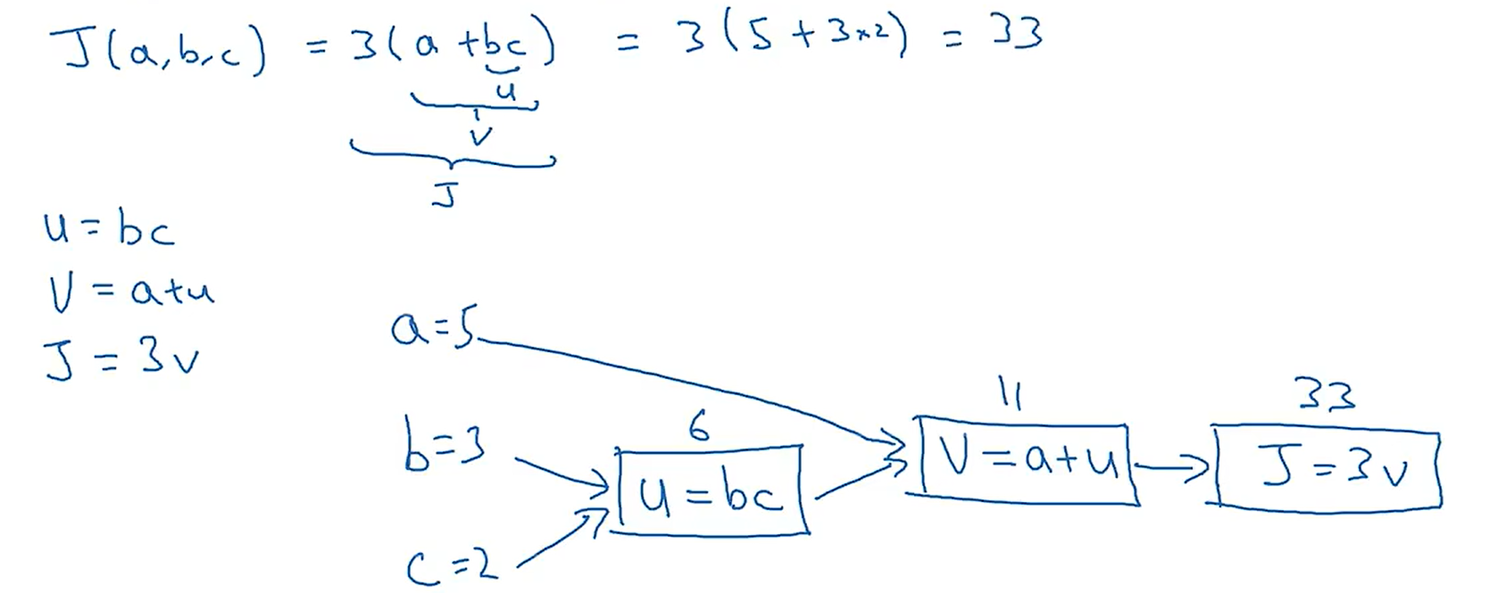
从上图可以看出,从左向右的过程,可以计算出J的值;那么从右向左的过程如下图所示:
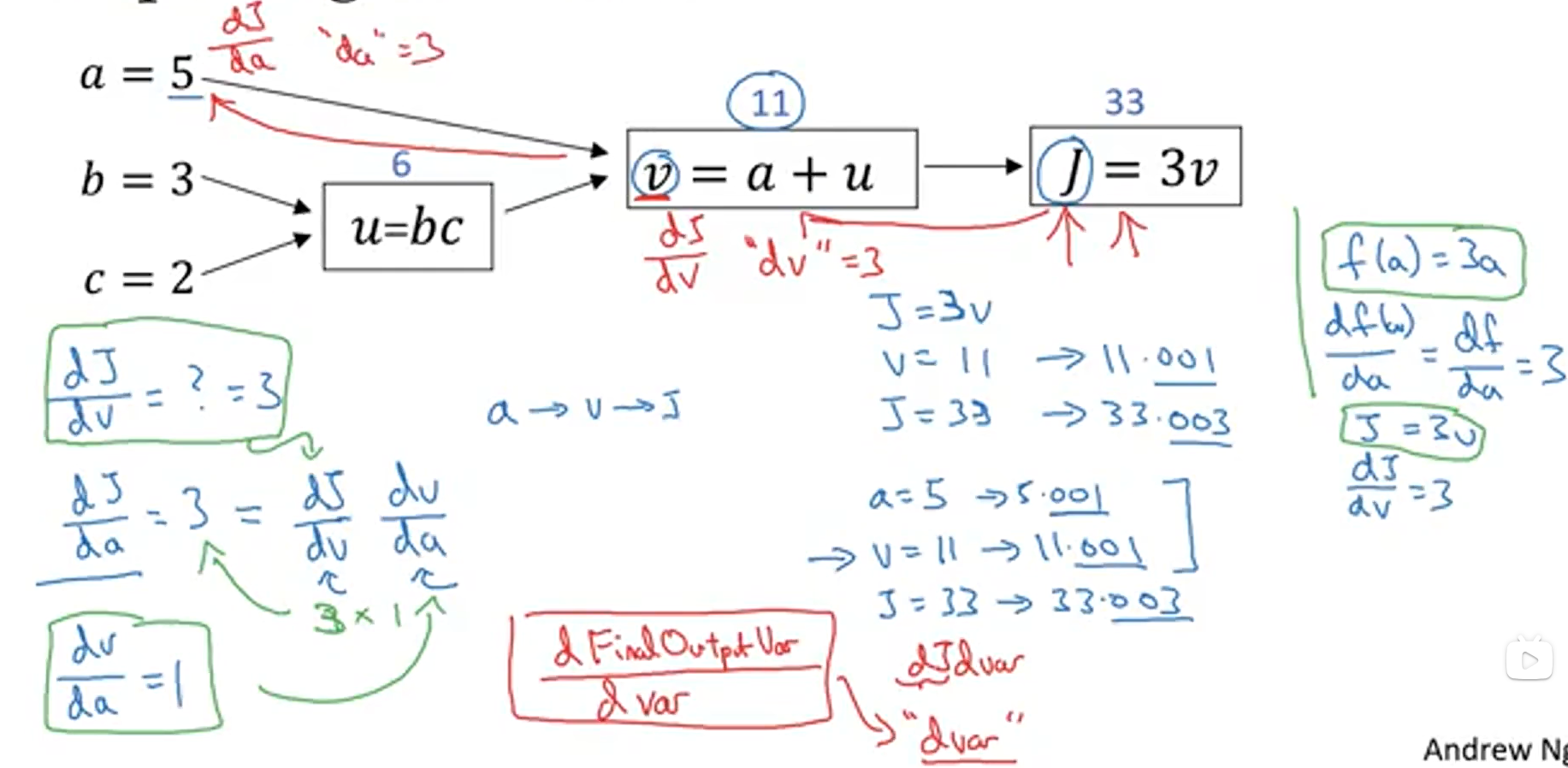
从右向左的计算过程,正对应着我们不断优化参数值,寻找最小J函数值的过程,我们知道计算一个函数的最小值,就是当这个函数的导数为0 的时候,因为我们的成本函数近似于一个凸函数,当导数为0时就对应着J函数的最小值。所以,从右向左的过程也就对应着计算导数的过程。
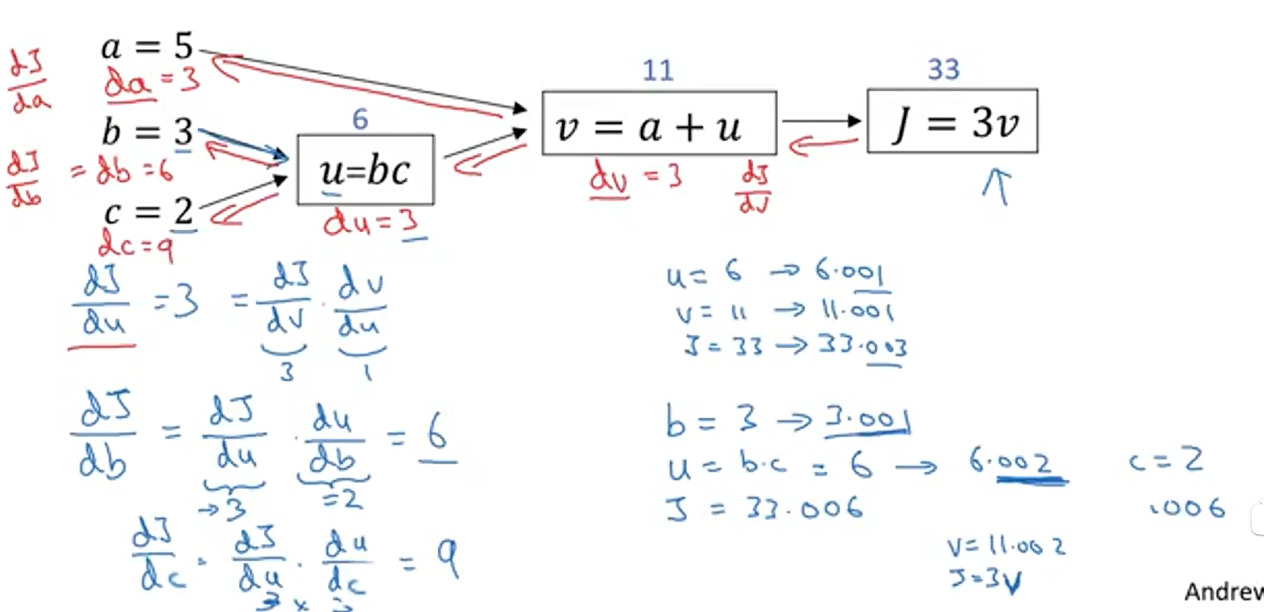
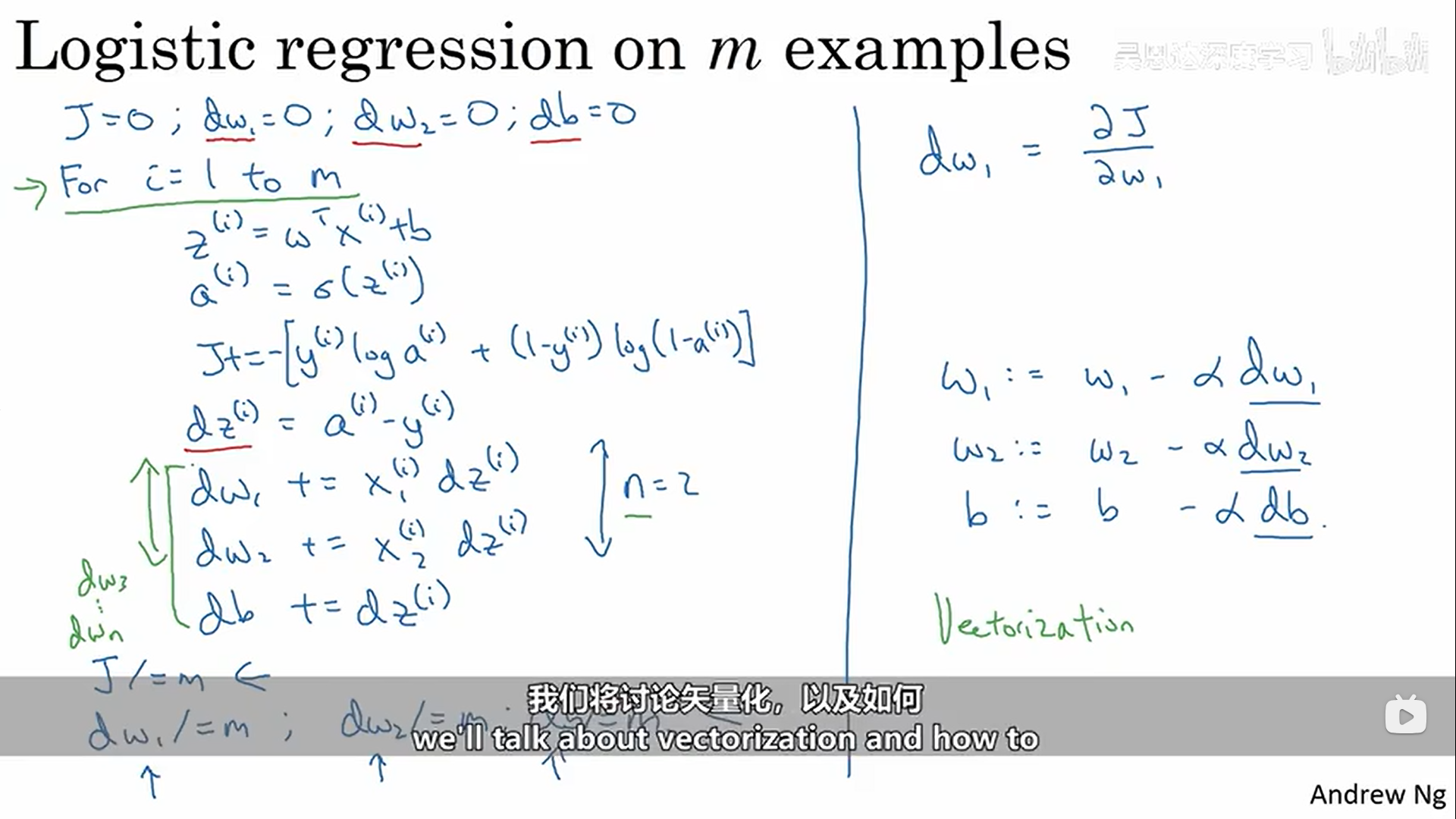
在从右向左的计算中,我们可以逐步计算出J函数对每一个变量的偏导数,从而便于我们对每一个变量进行梯度下降算法,找到最小的J函数值。下面是以逻辑回归的单个样本的梯度下降为实例讲解反向传播过程:
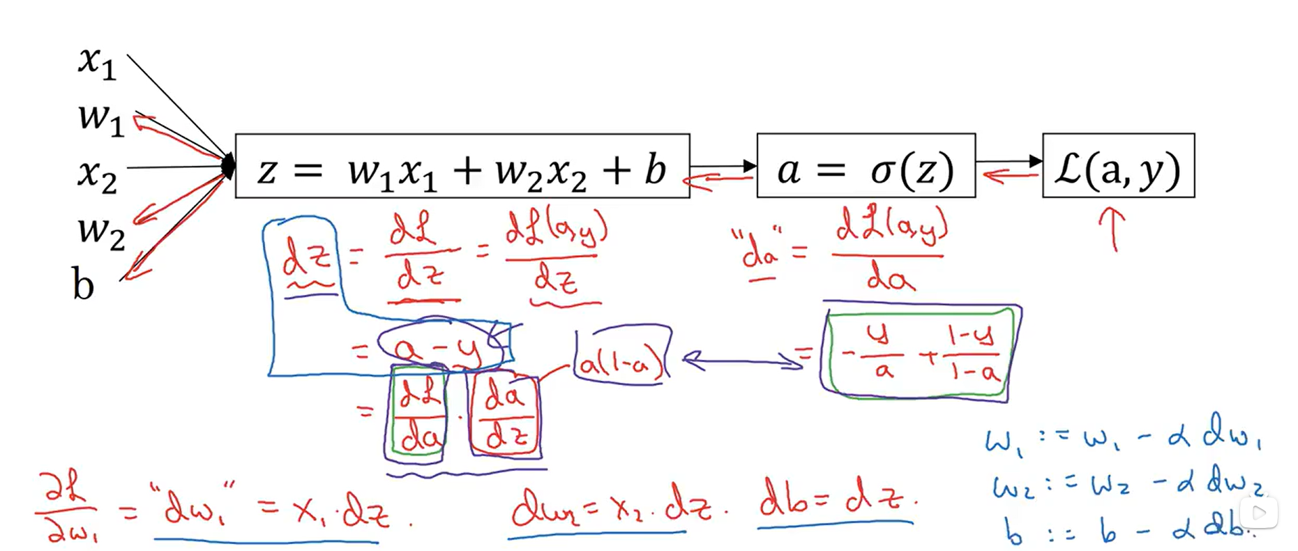
m的个样本的梯度下降,就是将所有样本关于参数的导数加起来求平均。
上述所有的示例,是为了让我们更好地理解正向传播和反向传播。
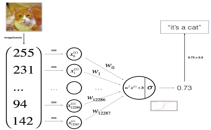
二、构建一个逻辑回归分类器来识别猫(使用神经网络思维)
(一)数据集
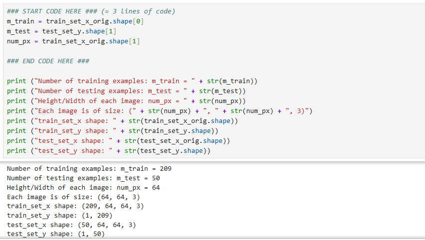
数据集("data.h5"),其中包含: - 标记为 cat (y=1) 或非 cat (y=0) 的 m_train 张图像的训练集 - 标记为 cat 或非 cat 的 m_test 张图像的测试集 - 每个图像的形状(num_px、num_px、3),其中 3 表示 3 个通道 (RGB)。因此,每个图像都是正方形(高度 = num_px)和(宽度 = num_px)。训练集、测试集、每一个样本图像的像素长度或者宽度。
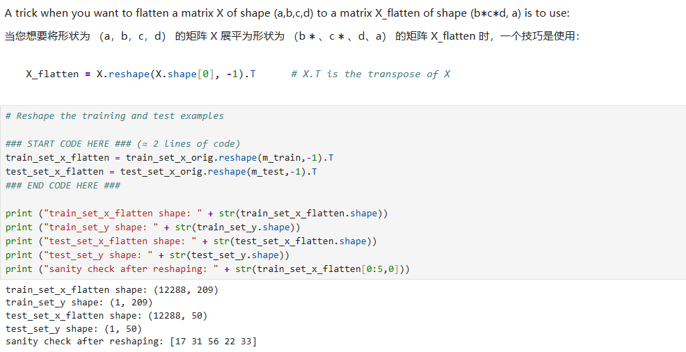
**对训练集和测试集特征进行矩阵形状的重塑:**在此之后,我们的训练(和测试)数据集是一个 numpy 数组,其中每列代表一个扁平化的图像。应该有 m_train 列(分别 m_test 列)。
**标准化数据:**机器学习中一个常见的预处理步骤是将数据集居中并标准化,这意味着您从每个示例中减去整个 numpy 数组的平均值,然后将每个示例除以整个 numpy 数组的标准差。但对于图片数据集,它更简单、更方便,并且只需将数据集的每一行除以 255(像素通道的最大值)几乎一样有效。
train_set_x = train_set_x_flatten/255.
test_set_x = test_set_x_flatten/255.
(二)使用神经网络思维方式构建逻辑回归
使用逻辑回归构建识别猫的模型的基本流程如下:
辅助函数sigmoid:
plain
def sigmoid(z):
     """
     Compute the sigmoid of z

     Arguments:
     z -- A scalar or numpy array of any size.

     Return:
     s -- sigmoid(z)
     """

     ### START CODE HERE ### (≈ 1 line of code)
     s = 1/(1+np.exp(-z))
     ### END CODE HERE ###

     return s
初始化参数:
plain
def initialize_with_zeros(dim):
     """
     This function creates a vector of zeros of shape (dim, 1) for w and initializes b to 0.

     Argument:
     dim -- size of the w vector we want (or number of parameters in this case)

     Returns:
     w -- initialized vector of shape (dim, 1)
     b -- initialized scalar (corresponds to the bias)
     """

     ### START CODE HERE ### (≈ 1 line of code)
     w = np.zeros((dim,1))
     b = 0
     ### END CODE HERE ###

     assert(w.shape == (dim, 1))
     assert(isinstance(b, float) or isinstance(b, int))

     return w, b
向前传播+向后传播:计算成本函数和梯度
plain
# GRADED FUNCTION: propagate

 def propagate(w, b, X, Y):
     """
     Implement the cost function and its gradient for the propagation explained above

     Arguments:
     w -- weights, a numpy array of size (num_px * num_px * 3, 1)
     b -- bias, a scalar
     X -- data of size (num_px * num_px * 3, number of examples)
     Y -- true "label" vector (containing 0 if non-cat, 1 if cat) of size (1, number of examples)

     Return:
     cost -- negative log-likelihood cost for logistic regression
     dw -- gradient of the loss with respect to w, thus same shape as w
     db -- gradient of the loss with respect to b, thus same shape as b

     Tips:
     - Write your code step by step for the propagation. np.log(), np.dot()
     """

     m = X.shape[1]

     # FORWARD PROPAGATION (FROM X TO COST)
     ### START CODE HERE ### (≈ 2 lines of code)
     y_pre = sigmoid(np.dot(w.T,X)+b)
     cost = np.sum(Y*np.log(y_pre)+(1-Y)*np.log(1-y_pre))/(-m)
     ### END CODE HERE ###

     # BACKWARD PROPAGATION (TO FIND GRAD)
     ### START CODE HERE ### (≈ 2 lines of code)
     dw = np.dot(X,(y_pre-Y).T)/m
     db = np.mean(y_pre-Y)

     ### END CODE HERE ###
     assert(dw.shape == w.shape)
     assert(db.dtype == float)
     cost = np.squeeze(cost)
     assert(cost.shape == ())

     grads = {"dw": dw,
              "db": db}

     return grads, cost
使用梯度下降来更新参数:
plain
# GRADED FUNCTION: optimize

 def optimize(w, b, X, Y, num_iterations, learning_rate, print_cost = False):
     """
     This function optimizes w and b by running a gradient descent algorithm

     Arguments:
     w -- weights, a numpy array of size (num_px * num_px * 3, 1)
     b -- bias, a scalar
     X -- data of shape (num_px * num_px * 3, number of examples)
     Y -- true "label" vector (containing 0 if non-cat, 1 if cat), of shape (1, number of examples)
     num_iterations -- number of iterations of the optimization loop
     learning_rate -- learning rate of the gradient descent update rule
     print_cost -- True to print the loss every 100 steps

     Returns:
     params -- dictionary containing the weights w and bias b
     grads -- dictionary containing the gradients of the weights and bias with respect to the cost function
     costs -- list of all the costs computed during the optimization, this will be used to plot the learning curve.

     Tips:
     You basically need to write down two steps and iterate through them:
         1) Calculate the cost and the gradient for the current parameters. Use propagate().
         2) Update the parameters using gradient descent rule for w and b.
     """

     costs = []

     for i in range(num_iterations):


         # Cost and gradient calculation (≈ 1-4 lines of code)
         ### START CODE HERE ###
         grads, cost = propagate(w, b, X, Y)
         ### END CODE HERE ###

         # Retrieve derivatives from grads
         dw = grads["dw"]
         db = grads["db"]

         # update rule (≈ 2 lines of code)
         ### START CODE HERE ###
         w = w - dw*learning_rate
         b = b - db*learning_rate
         ### END CODE HERE ###

         # Record the costs
         if i % 100 == 0:
             costs.append(cost)

         # Print the cost every 100 training examples
         if print_cost and i % 100 == 0:
             print ("Cost after iteration %i: %f" %(i, cost))

     params = {"w": w,
               "b": b}

     grads = {"dw": dw,
              "db": db}

     return params, grads, costs
使用优化之后的参数进行预测:
plain
# GRADED FUNCTION: predict

 def predict(w, b, X):
     '''
     Predict whether the label is 0 or 1 using learned logistic regression parameters (w, b)

     Arguments:
     w -- weights, a numpy array of size (num_px * num_px * 3, 1)
     b -- bias, a scalar
     X -- data of size (num_px * num_px * 3, number of examples)

     Returns:
     Y_prediction -- a numpy array (vector) containing all predictions (0/1) for the examples in X
     '''

     m = X.shape[1]
     Y_prediction = np.zeros((1,m))
     w = w.reshape(X.shape[0], 1)

     # Compute vector "A" predicting the probabilities of a cat being present in the picture
     ### START CODE HERE ### (≈ 1 line of code)
     A = np.dot(w.T,X)+b
     ### END CODE HERE ###

     for i in range(A.shape[1]):

         # Convert probabilities A[0,i] to actual predictions p[0,i]
         ### START CODE HERE ### (≈ 4 lines of code)
         if(A[0][i]<=0.5):
             Y_prediction[0][i] = 0
         else:
             Y_prediction[0][i] = 1
         ### END CODE HERE ###

     assert(Y_prediction.shape == (1, m))

     return Y_prediction
将所有的函数合并到一个模型中:
plain
def model(X_train, Y_train, X_test, Y_test, num_iterations = 2000, learning_rate = 0.5, print_cost = False):
     """
     Builds the logistic regression model by calling the function you've implemented previously

     Arguments:
     X_train -- training set represented by a numpy array of shape (num_px * num_px * 3, m_train)
     Y_train -- training labels represented by a numpy array (vector) of shape (1, m_train)
     X_test -- test set represented by a numpy array of shape (num_px * num_px * 3, m_test)
     Y_test -- test labels represented by a numpy array (vector) of shape (1, m_test)
     num_iterations -- hyperparameter representing the number of iterations to optimize the parameters
     learning_rate -- hyperparameter representing the learning rate used in the update rule of optimize()
     print_cost -- Set to true to print the cost every 100 iterations

     Returns:
     d -- dictionary containing information about the model.
     """

     ### START CODE HERE ###

     # initialize parameters with zeros (≈ 1 line of code)
     w,b = initialize_with_zeros(X_train.shape[0])
     # Gradient descent (≈ 1 line of code)
     grads,cost = propagate(w, b, X_train, Y_train)

     # Retrieve parameters w and b from dictionary "parameters"
     params, grads, costs = optimize(w, b, X_train, Y_train, num_iterations, learning_rate, print_cost)
     w = params["w"]
     b = params["b"]

     # Predict test/train set examples (≈ 2 lines of code)
     Y_prediction_test = predict(w, b, X_test)
     Y_prediction_train = predict(w, b, X_train)

     ### END CODE HERE ###

     # Print train/test Errors
     print("train accuracy: {} %".format(100 - np.mean(np.abs(Y_prediction_train - Y_train)) * 100))
     print("test accuracy: {} %".format(100 - np.mean(np.abs(Y_prediction_test - Y_test)) * 100))


     d = {"costs": costs,
          "Y_prediction_test": Y_prediction_test,
          "Y_prediction_train" : Y_prediction_train,
          "w" : w,
          "b" : b,
          "learning_rate" : learning_rate,
          "num_iterations": num_iterations}

     return d
总结;1.预处理数据集很重要。2. 分别实现了每个函数:initialize()、propagate()、optimize()。然后构建了一个 model()。3. 调整学习率(这是"超参数"的一个例子)可以对算法产生很大的影响。
最后,防止过拟合可以加入正则化项,学习率的选择可以使用动态优化学习率函数。机器学习课程中都有讲过。