计算机专业的你懂的：大数据毕设就选贵州茅台股票分析系统准没错|计算机毕业设计|数据可视化|数据分析

前言

💖💖作者：计算机程序员小杨
💙💙个人简介：我是一名计算机相关专业的从业者，擅长Java、微信小程序、Python、Golang、安卓Android等多个IT方向。会做一些项目定制化开发、代码讲解、答辩教学、文档编写、也懂一些降重方面的技巧。热爱技术，喜欢钻研新工具和框架，也乐于通过代码解决实际问题，大家有技术代码这一块的问题可以问我！
💛💛想说的话：感谢大家的关注与支持！
💕💕文末获取源码联系计算机程序员小杨
💜💜
网站实战项目
安卓/小程序实战项目
大数据实战项目
深度学习实战项目
计算机毕业设计选题
💜💜

一.开发工具简介

大数据框架：Hadoop+Spark（本次没用Hive，支持定制）
开发语言：Python+Java（两个版本都支持）
后端框架：Django+Spring Boot(Spring+SpringMVC+Mybatis)（两个版本都支持）
前端：Vue+ElementUI+Echarts+HTML+CSS+JavaScript+jQuery
详细技术点：Hadoop、HDFS、Spark、Spark SQL、Pandas、NumPy
数据库：MySQL

二.系统内容简介

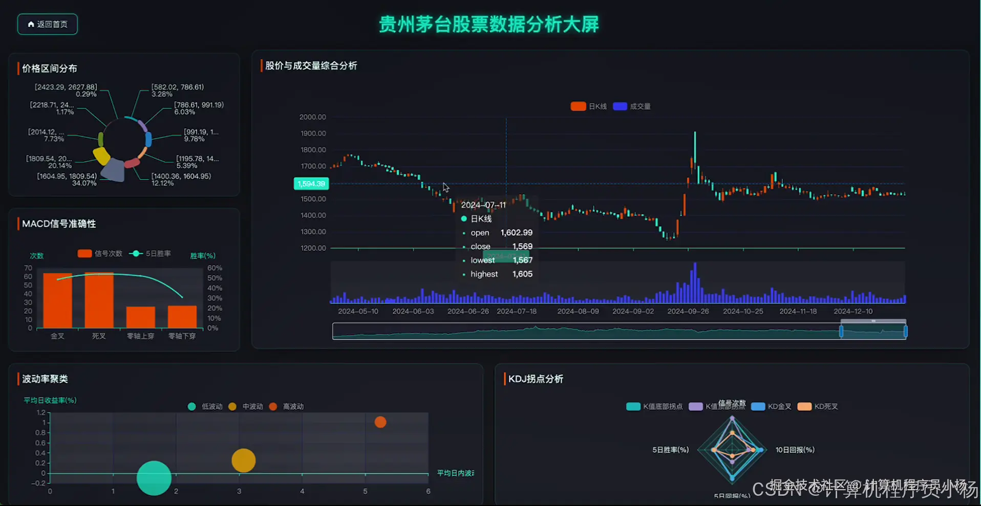
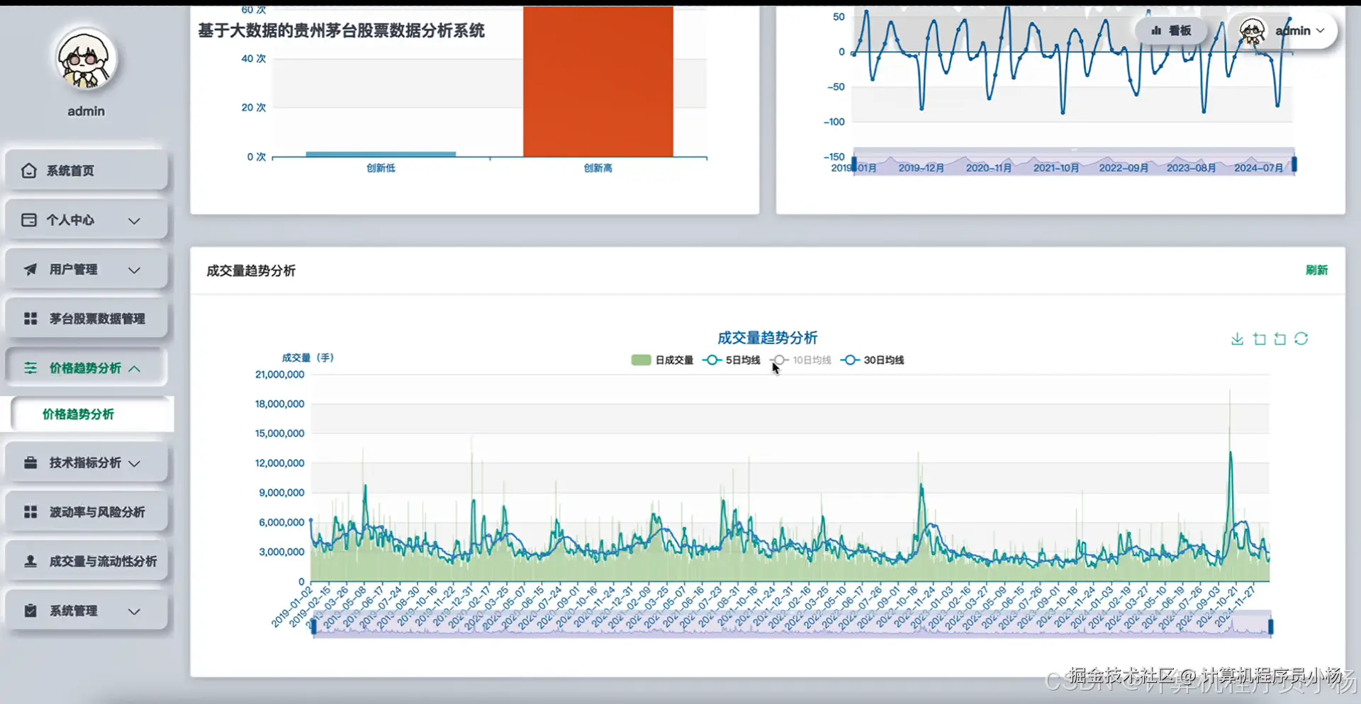
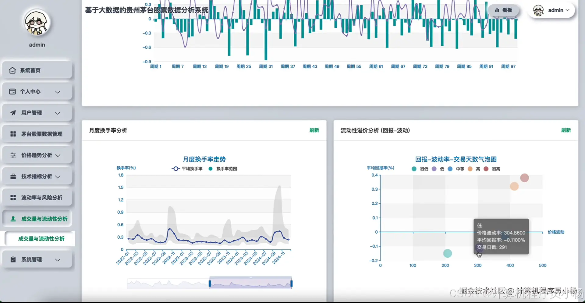
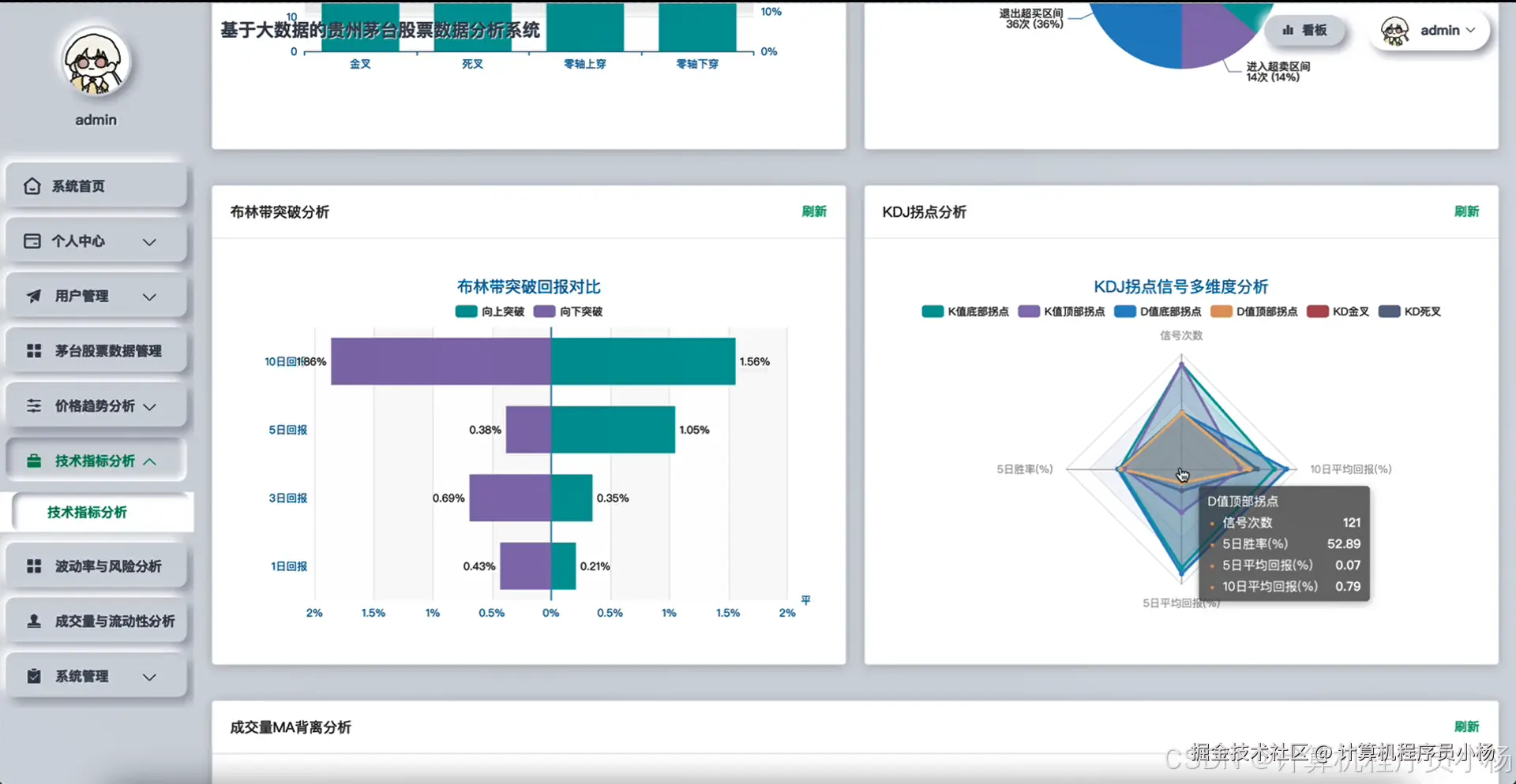
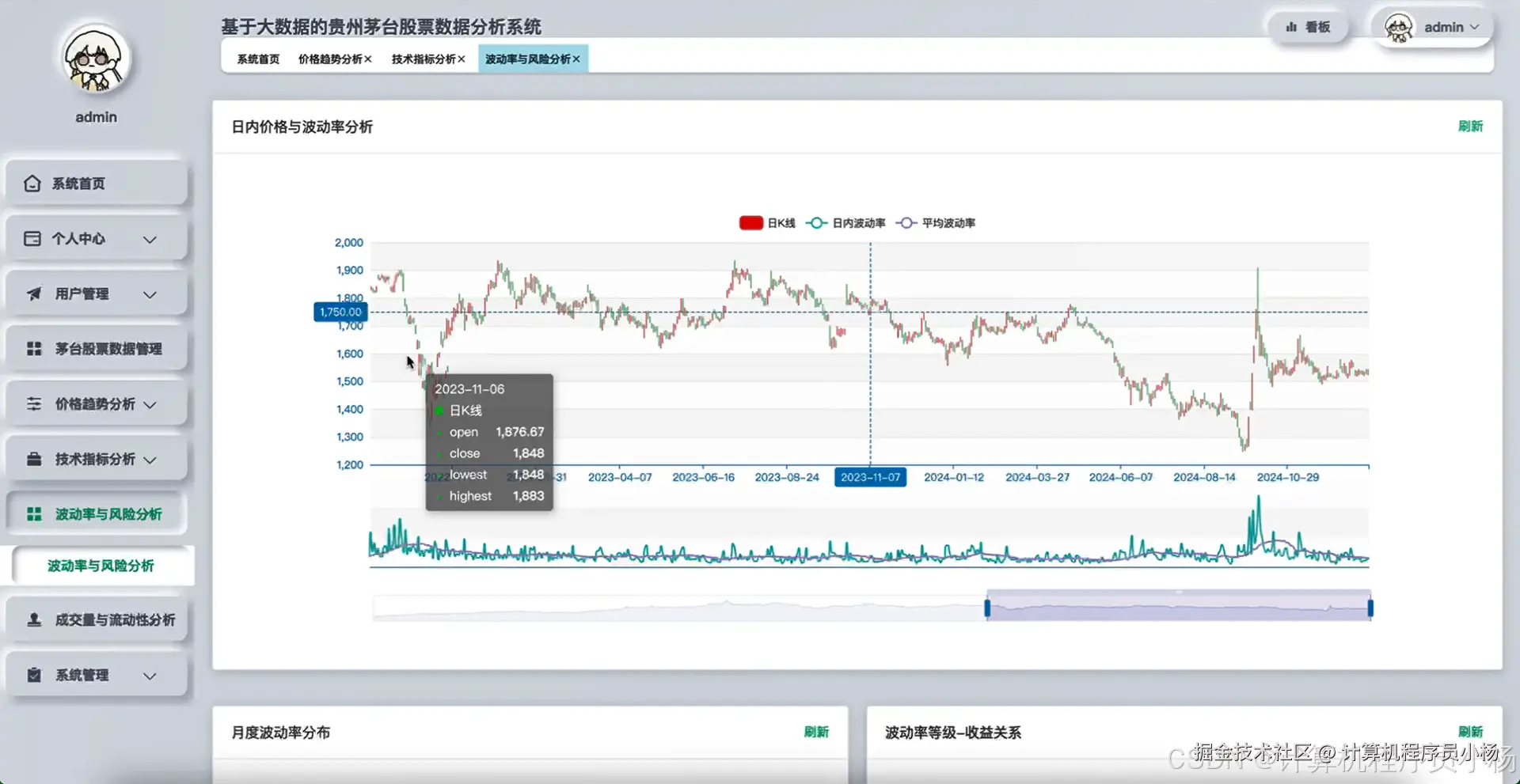
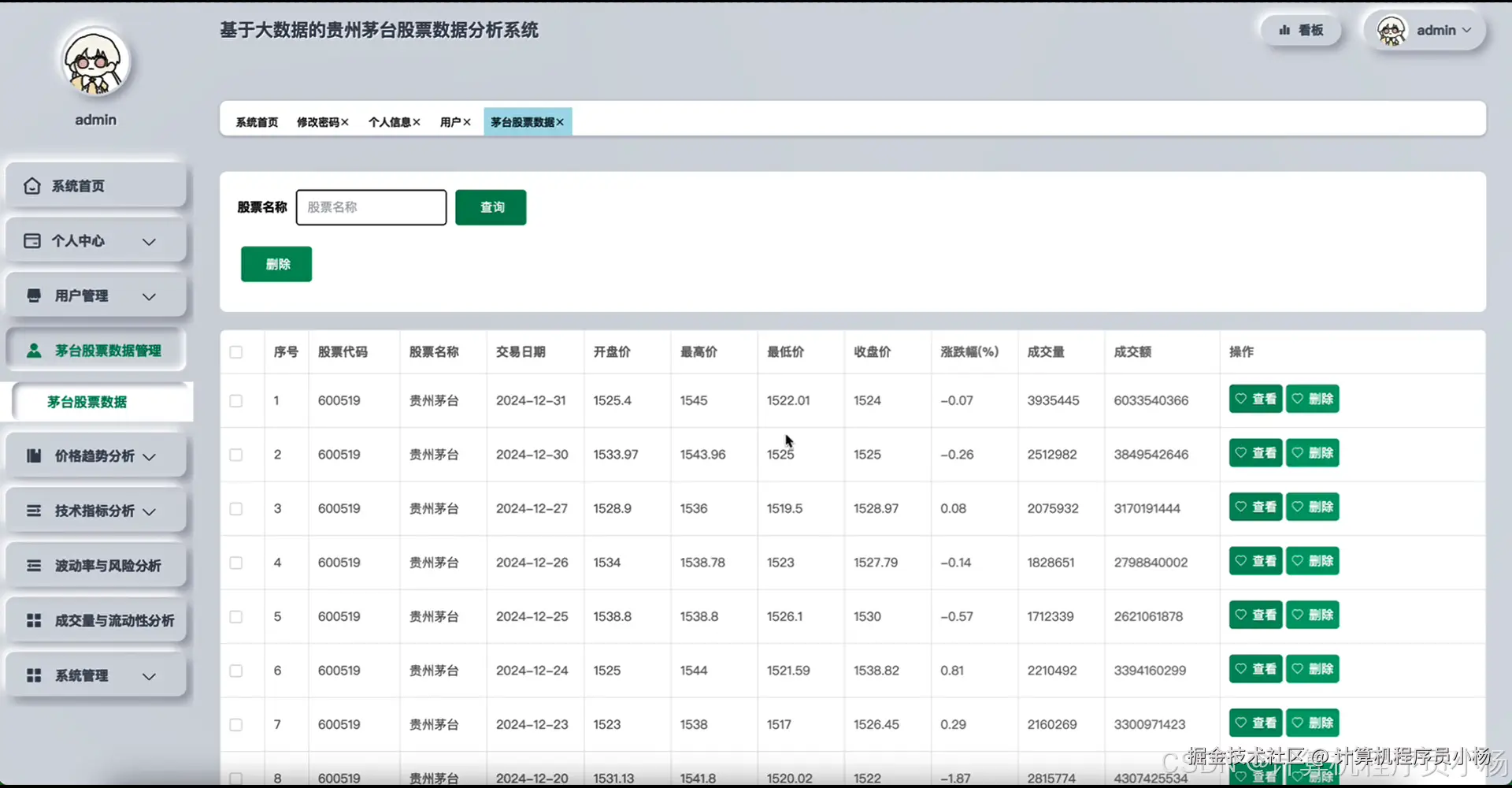
基于大数据的贵州茅台股票数据分析系统是一个集数据采集、存储、处理和可视化分析于一体的综合性股票分析平台。系统采用Hadoop分布式文件系统作为底层数据存储架构，通过Spark大数据处理框架实现对茅台股票海量历史数据的高效分析处理。在技术实现层面，系统提供Python和Java双语言版本支持，后端分别采用Django和Spring Boot框架构建RESTful API接口，前端运用Vue.js结合ElementUI组件库打造现代化用户界面，通过ECharts图表库实现数据的直观可视化展示。系统核心功能涵盖茅台股票基础数据管理、价格趋势深度分析、技术指标计算、波动率与风险评估、成交量与流动性分析等多个维度，通过Spark SQL进行复杂查询处理，结合Pandas和NumPy进行数据科学计算，为用户提供全方位的股票分析服务。整个系统架构设计合理，技术栈搭配完善，既能满足大数据处理需求，又具备良好的用户体验和系统扩展性。

三.系统功能演示

计算机专业的你懂的：大数据毕设就选贵州茅台股票分析系统准没错|计算机毕业设计|数据可视化|数据分析

四.系统界面展示

五.系统源码展示

css 复制代码

from pyspark.sql import SparkSession
from pyspark.sql.functions import *
from pyspark.sql.types import *
import pandas as pd
import numpy as np

spark = SparkSession.builder.appName("MaotaiStockAnalysis").config("spark.sql.adaptive.enabled", "true").getOrCreate()

def price_trend_analysis(stock_data):
    df = spark.createDataFrame(stock_data)
    df.createOrReplaceTempView("stock_temp")
    trend_result = spark.sql("""
        SELECT 
            trade_date,
            close_price,
            open_price,
            high_price,
            low_price,
            LAG(close_price, 1) OVER (ORDER BY trade_date) as prev_close,
            (close_price - LAG(close_price, 1) OVER (ORDER BY trade_date)) / LAG(close_price, 1) OVER (ORDER BY trade_date) * 100 as daily_return,
            AVG(close_price) OVER (ORDER BY trade_date ROWS BETWEEN 4 PRECEDING AND CURRENT ROW) as ma5,
            AVG(close_price) OVER (ORDER BY trade_date ROWS BETWEEN 9 PRECEDING AND CURRENT ROW) as ma10,
            AVG(close_price) OVER (ORDER BY trade_date ROWS BETWEEN 19 PRECEDING AND CURRENT ROW) as ma20,
            CASE 
                WHEN close_price > LAG(close_price, 1) OVER (ORDER BY trade_date) THEN 'UP'
                WHEN close_price < LAG(close_price, 1) OVER (ORDER BY trade_date) THEN 'DOWN'
                ELSE 'FLAT'
            END as trend_direction
        FROM stock_temp
        ORDER BY trade_date
    """)
    trend_pandas = trend_result.toPandas()
    trend_pandas['price_momentum'] = trend_pandas['daily_return'].rolling(window=5).mean()
    trend_pandas['volatility_index'] = trend_pandas['daily_return'].rolling(window=10).std() * 100
    trend_analysis = {
        'trend_data': trend_pandas.to_dict('records'),
        'avg_daily_return': float(trend_pandas['daily_return'].mean()),
        'max_single_gain': float(trend_pandas['daily_return'].max()),
        'max_single_loss': float(trend_pandas['daily_return'].min()),
        'trend_consistency': len(trend_pandas[trend_pandas['trend_direction'] == trend_pandas['trend_direction'].mode()[0]]) / len(trend_pandas)
    }
    return trend_analysis

def technical_indicator_analysis(stock_data):
    df = spark.createDataFrame(stock_data)
    df.createOrReplaceTempView("technical_temp")
    rsi_result = spark.sql("""
        SELECT 
            trade_date,
            close_price,
            close_price - LAG(close_price, 1) OVER (ORDER BY trade_date) as price_change,
            CASE 
                WHEN close_price - LAG(close_price, 1) OVER (ORDER BY trade_date) > 0 
                THEN close_price - LAG(close_price, 1) OVER (ORDER BY trade_date) 
                ELSE 0 
            END as gain,
            CASE 
                WHEN close_price - LAG(close_price, 1) OVER (ORDER BY trade_date) < 0 
                THEN ABS(close_price - LAG(close_price, 1) OVER (ORDER BY trade_date)) 
                ELSE 0 
            END as loss,
            high_price,
            low_price,
            volume
        FROM technical_temp
        ORDER BY trade_date
    """)
    technical_pandas = rsi_result.toPandas()
    technical_pandas['avg_gain'] = technical_pandas['gain'].rolling(window=14).mean()
    technical_pandas['avg_loss'] = technical_pandas['loss'].rolling(window=14).mean()
    technical_pandas['rs'] = technical_pandas['avg_gain'] / (technical_pandas['avg_loss'] + 0.000001)
    technical_pandas['rsi'] = 100 - (100 / (1 + technical_pandas['rs']))
    technical_pandas['highest_high'] = technical_pandas['high_price'].rolling(window=14).max()
    technical_pandas['lowest_low'] = technical_pandas['low_price'].rolling(window=14).min()
    technical_pandas['k_percent'] = ((technical_pandas['close_price'] - technical_pandas['lowest_low']) / (technical_pandas['highest_high'] - technical_pandas['lowest_low'])) * 100
    technical_pandas['d_percent'] = technical_pandas['k_percent'].rolling(window=3).mean()
    ema_12 = technical_pandas['close_price'].ewm(span=12).mean()
    ema_26 = technical_pandas['close_price'].ewm(span=26).mean()
    technical_pandas['macd_line'] = ema_12 - ema_26
    technical_pandas['signal_line'] = technical_pandas['macd_line'].ewm(span=9).mean()
    technical_pandas['macd_histogram'] = technical_pandas['macd_line'] - technical_pandas['signal_line']
    technical_indicators = {
        'indicator_data': technical_pandas[['trade_date', 'rsi', 'k_percent', 'd_percent', 'macd_line', 'signal_line', 'macd_histogram']].to_dict('records'),
        'current_rsi': float(technical_pandas['rsi'].iloc[-1]) if len(technical_pandas) > 0 else 0,
        'rsi_overbought_signals': len(technical_pandas[technical_pandas['rsi'] > 70]),
        'rsi_oversold_signals': len(technical_pandas[technical_pandas['rsi'] < 30]),
        'macd_bullish_crossovers': len(technical_pandas[(technical_pandas['macd_line'] > technical_pandas['signal_line']) & (technical_pandas['macd_line'].shift(1) <= technical_pandas['signal_line'].shift(1))]),
        'macd_bearish_crossovers': len(technical_pandas[(technical_pandas['macd_line'] < technical_pandas['signal_line']) & (technical_pandas['macd_line'].shift(1) >= technical_pandas['signal_line'].shift(1))])
    }
    return technical_indicators

def volatility_risk_analysis(stock_data):
    df = spark.createDataFrame(stock_data)
    df.createOrReplaceTempView("volatility_temp")
    volatility_result = spark.sql("""
        SELECT 
            trade_date,
            close_price,
            high_price,
            low_price,
            (close_price - LAG(close_price, 1) OVER (ORDER BY trade_date)) / LAG(close_price, 1) OVER (ORDER BY trade_date) as daily_return,
            ((high_price - low_price) / close_price) * 100 as daily_range_pct,
            volume,
            volume * close_price as turnover_value
        FROM volatility_temp
        ORDER BY trade_date
    """)
    volatility_pandas = volatility_result.toPandas()
    volatility_pandas['return_squared'] = volatility_pandas['daily_return'] ** 2
    volatility_pandas['historical_volatility'] = volatility_pandas['daily_return'].rolling(window=20).std() * np.sqrt(252) * 100
    volatility_pandas['rolling_var'] = volatility_pandas['daily_return'].rolling(window=30).var()
    volatility_pandas['price_deviation'] = abs(volatility_pandas['close_price'] - volatility_pandas['close_price'].rolling(window=20).mean()) / volatility_pandas['close_price'].rolling(window=20).mean() * 100
    cumulative_returns = (1 + volatility_pandas['daily_return'] / 100).cumprod() - 1
    rolling_max = cumulative_returns.expanding().max()
    volatility_pandas['drawdown'] = (cumulative_returns - rolling_max) * 100
    volatility_pandas['max_drawdown'] = volatility_pandas['drawdown'].expanding().min()
    var_95 = np.percentile(volatility_pandas['daily_return'].dropna(), 5)
    var_99 = np.percentile(volatility_pandas['daily_return'].dropna(), 1)
    avg_return = volatility_pandas['daily_return'].mean()
    return_std = volatility_pandas['daily_return'].std()
    sharpe_ratio = (avg_return / return_std) * np.sqrt(252) if return_std != 0 else 0
    downside_returns = volatility_pandas['daily_return'][volatility_pandas['daily_return'] < 0]
    downside_std = downside_returns.std() if len(downside_returns) > 0 else 0
    sortino_ratio = (avg_return / downside_std) * np.sqrt(252) if downside_std != 0 else 0
    risk_metrics = {
        'volatility_data': volatility_pandas[['trade_date', 'daily_return', 'historical_volatility', 'drawdown', 'max_drawdown', 'daily_range_pct']].to_dict('records'),
        'current_volatility': float(volatility_pandas['historical_volatility'].iloc[-1]) if len(volatility_pandas) > 0 else 0,
        'var_95': float(var_95),
        'var_99': float(var_99),
        'max_historical_drawdown': float(volatility_pandas['max_drawdown'].min()),
        'sharpe_ratio': float(sharpe_ratio),
        'sortino_ratio': float(sortino_ratio),
        'volatility_trend': 'INCREASING' if volatility_pandas['historical_volatility'].iloc[-5:].mean() > volatility_pandas['historical_volatility'].iloc[-10:-5].mean() else 'DECREASING'
    }
    return risk_metrics

六.系统文档展示

结束

💛💛想说的话：感谢大家的关注与支持！
💕💕文末获取源码联系计算机程序员小杨
💜💜
网站实战项目
安卓/小程序实战项目
大数据实战项目
深度学习实战项目
计算机毕业设计选题
💜💜