华大时空组学空转图像处理
library(png)
library(tiff)
st <- readRDS('01.Stereo-seq/output_all/Demo_Mouse_Kidney/outs/feature_expression/seurat_out.rds')
dim(st@assays$Spatial@counts)
st@assays$Spatial@counts[1:4,1:4]
coord.df <- data.frame(imagerow = st$x, imagecol=st$y,nCount_Spatial = st$nCount_Spatial,row.names = st$X_index)
min(coord.df$imagerow);max(coord.df$imagerow);min(coord.df$imagecol);max(coord.df$imagecol)
#image <- readPNG(source = '/public/user/huguang/st-seq/down_string_pipline/bin1_img_tissue_cut.png')
image <- readTIFF("/biodata2/08.user/zhengyzh/01.Stereo-seq/output_all/Demo_Mouse_Kidney/outs/image/bin1_img_tissue_cut.tif")
用于seurat
st@images$slice1  = new(
  Class = 'SlideSeq',
  assay = "Spatial",
  key = "image_",
  #image = image,
  coordinates = coord.df
)
图像分bin转化
bin_matrix_fast <- function(mat, bin_size=200) {
  n <- nrow(mat)
  m <- ncol(mat)

  # 修剪矩阵以适应bin大小
  trimmed_n <- floor(n / bin_size) * bin_size
  trimmed_m <- floor(m / bin_size) * bin_size
  mat <- mat[1:trimmed_n, 1:trimmed_m]

  # 重新塑造矩阵
  dim(mat) <- c(bin_size, trimmed_n/bin_size, bin_size, trimmed_m/bin_size)

  # 计算每个bin的均值
  result <- apply(mat, c(2, 4), mean, na.rm = TRUE)

  return(result)
}

img <- bin_matrix_fast(image, 50)
img <- img[dim(img)[1]:1,] # 实现图像的上下翻转
# SpatialDimPlot(st)
# SpatialFeaturePlot(st, features = "nCount_Spatial")
# SpatialFeaturePlot(st, features = "ENSMUSG00000000028",cols = ifelse(st@assays$Spatial@counts['ENSMUSG00000000028',]>0,'red','gray'))
# st@reductions$spatial@cell.embeddings
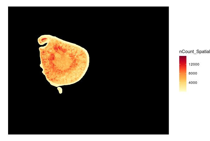
ggplot2手搓实现切片图像背景图效果
ggplot() +
  #背景图片
  annotation_raster(img, 0, dim(img)[1], 0, dim(img)[2]) + # 此处也可转化为0,1的标准化数值,需下面point同步修改
  geom_point(data = coord.df, aes(x=imagerow/50,y=imagecol/50,color=nCount_Spatial)) +
  scale_color_gradientn(colours = RColorBrewer::brewer.pal(9,'YlOrRd')) +
  xlim(0,dim(img)[1]) + ylim(0,dim(img)[2]) +
  theme_void()
# 标准灰度转换公式:0.299*R + 0.587*G + 0.114*B
gray_img <- 0.299 * img[,,1] + 0.587 * img[,,2] + 0.114 * img[,,3] # 注意这里是 R G B 图像矩阵*权重的加和,3变1

# 显示灰度图
grid.raster(gray_img, interpola = TRUE)

# 或者保存为单通道数组
gray_array <- array(gray_img, dim = c(dim(img)[1], dim(img)[2], 1))