人工智能机器学习——逻辑回归

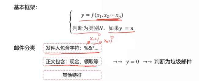
一、分类问题(Classification)

垃圾邮件检测

流程

标注样本邮件未垃圾/普通邮件（人)

获取批量的样本邮件及其标签，学习其特征（计算机）

针对新的邮件，自动判断其类别（计算机）

图像分类

数字识别

分类

分类：根据已知样本的某些特征，判断一个新的样本属于哪种已知的样本类

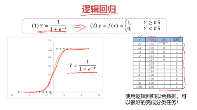
二、分类方法

逻辑回归
KNN近邻模型
决策树
神经网络

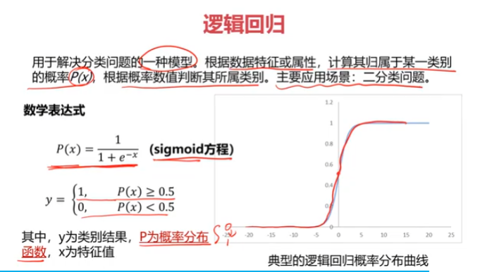
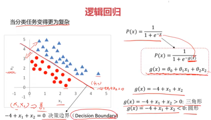
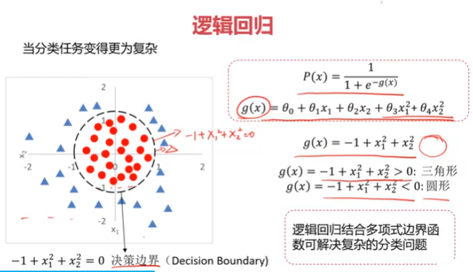
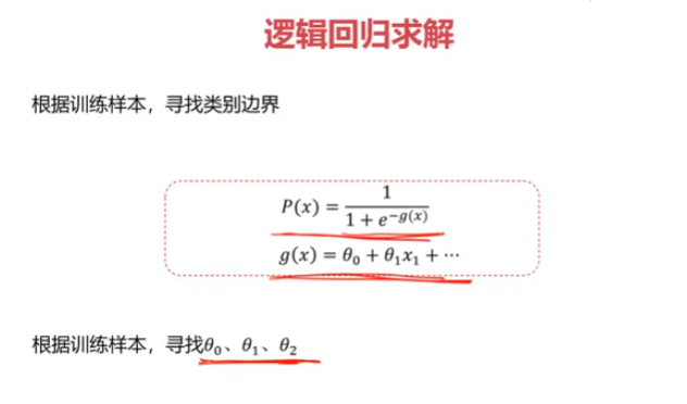
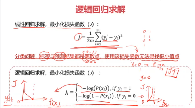
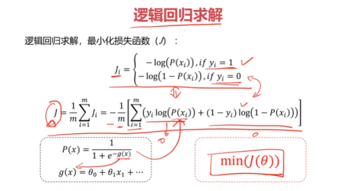
逻辑回归

三、考试通过预测，使用数据集examdata.csv

复制代码

#加载数据
import pandas as pd
import numpy as np
data = pd.read_csv('examdata.csv')
data.head()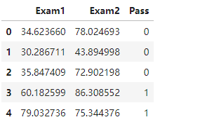

复制代码

#画散点图
from matplotlib import pyplot as plt
fig1 = plt.figure()
plt.scatter(data.loc[:,'Exam1'],data.loc[:,'Exam2'])
plt.title("Exam1-Exam2")
plt.xlabel("Exam1")
plt.ylabel("Exam2")
plt.show()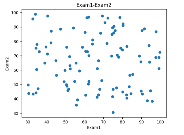

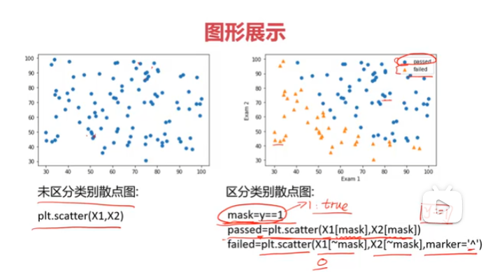
复制代码

#区分数据
mask = data.loc[:,'Pass']==1
print(mask)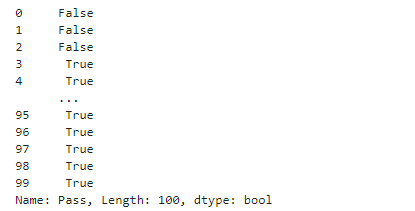

复制代码

fig2 = plt.figure()
passed = plt.scatter(data.loc[:,'Exam1'][mask],data.loc[:,'Exam2'][mask])
failed = plt.scatter(data.loc[:,'Exam1'][~mask],data.loc[:,'Exam2'][~mask])
plt.title("Exam1-Exam2")
plt.xlabel("Exam1")
plt.ylabel("Exam2")
plt.legend((passed,failed),("passed","failed"))
plt.show()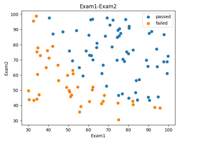

复制代码

#赋值x，y
x = data.drop(['Pass'],axis=1)
x.head()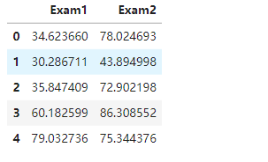

复制代码

x1 = data.loc[:,'Exam1']
x2 = data.loc[:,'Exam2']

y = data.loc[:,'Pass']
y.head()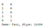

复制代码

#打印x,y维度
print(x.shape,y.shape)

复制代码

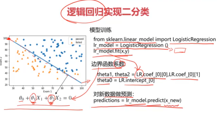
#训练逻辑回归模型
from sklearn.linear_model import LogisticRegression
LR = LogisticRegression()
LR.fit(x,y)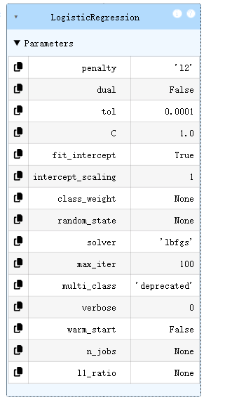

复制代码

#预测结果
y_predict = LR.predict(x)
print(y_predict)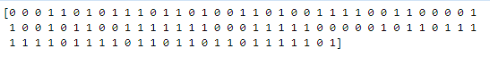

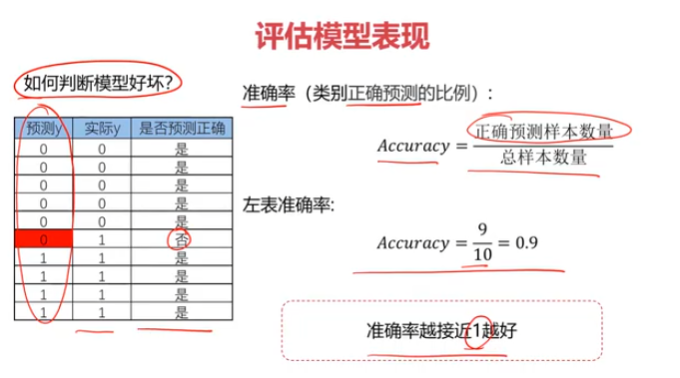
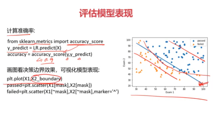
复制代码

#打印预测准确率
from sklearn.metrics import accuracy_score
accuracy = accuracy_score(y,y_predict)
print(accuracy)

复制代码

#预测新数据
X_test = pd.DataFrame([[70,65]],columns=['Exam1','Exam2'])
y_test = LR.predict(X_test)
print('passed' if y_test==1 else 'failed')

复制代码

#边界曲线
LR.coef_

复制代码

LR.intercept_

复制代码

theta0 = LR.intercept_
theta1,theta2 = LR.coef_[0][0],LR.coef_[0][1]
print(theta0,theta1,theta2)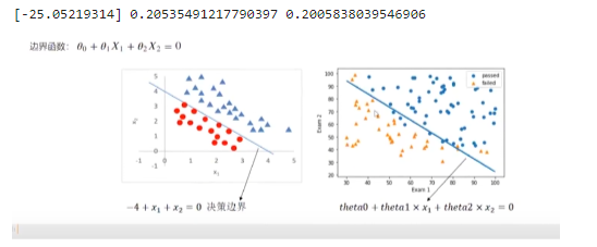

复制代码

X2_new = -(theta0+theta1*x1)/theta2
print(X2_new)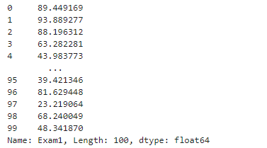

复制代码

fig3 = plt.figure()
passed = plt.scatter(data.loc[:,'Exam1'][mask],data.loc[:,'Exam2'][mask])
failed = plt.scatter(data.loc[:,'Exam1'][~mask],data.loc[:,'Exam2'][~mask])
plt.plot(x1,X2_new)
plt.title("Exam1-Exam2")
plt.xlabel("Exam1")
plt.ylabel("Exam2")
plt.legend((passed,failed),("passed","failed"))
plt.show()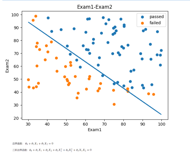

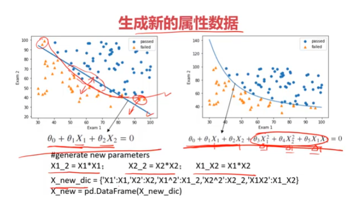
复制代码

#使用二阶边界函数
X1_2 = x1*x1
X2_2 = x2*x2
X1_X2 = x1*x2

X_new = {'X1':x1,'X2':x2,'X1_2':X1_2,'X2_2':X2_2,'X1_X2':X1_X2}
X_new = pd.DataFrame(X_new)
print(X_new)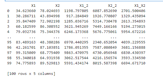

复制代码

#创建模型2
LR2 = LogisticRegression(solver='liblinear', max_iter=1000)# solver='saga',    # 最通用的求解器 max_iter=1000,    # 足够的迭代次数
LR2.fit(X_new,y)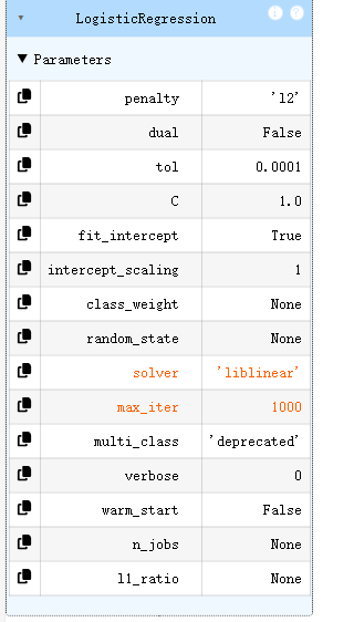

复制代码

#预测结果
y_2_predict = LR2.predict(X_new)
print(y_2_predict)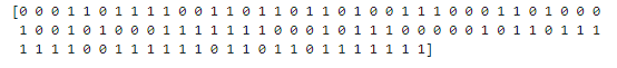

复制代码

#打印预测准确率
accuracy = accuracy_score(y,y_2_predict)
print(accuracy)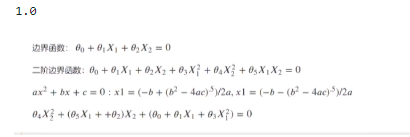

复制代码

#对x1排序
X1_new = x1.sort_values()
print(x1,X1_new)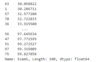

复制代码

LR2.coef_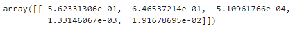

复制代码

theta0 = LR2.intercept_
theta1,theta2,theta3,theta4,theta5 = LR2.coef_[0][0],LR2.coef_[0][1],LR2.coef_[0][2],LR2.coef_[0][3],LR2.coef_[0][4]
a = theta4
b = theta5*X1_new+theta2
c = theta0+theta1*X1_new+theta3*X1_new*X1_new
X2_new_boundary = (-b+np.sqrt(b*b-4*a*c))/(2*a)

print(theta0,theta1,theta2,theta3,theta4,theta5)
print(X2_new_boundary)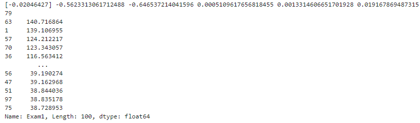

复制代码

fig4 = plt.figure()
plt.plot(x1,X2_new_boundary)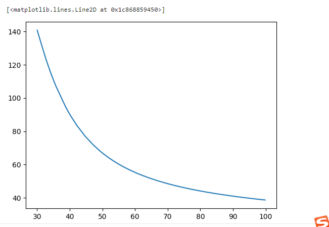

复制代码

fig5 = plt.figure()
passed = plt.scatter(data.loc[:,'Exam1'][mask],data.loc[:,'Exam2'][mask])
failed = plt.scatter(data.loc[:,'Exam1'][~mask],data.loc[:,'Exam2'][~mask])
plt.plot(x1,X2_new_boundary)
plt.title("Exam1-Exam2")
plt.xlabel("Exam1")
plt.ylabel("Exam2")
plt.legend((passed,failed),("passed","failed"))
plt.show()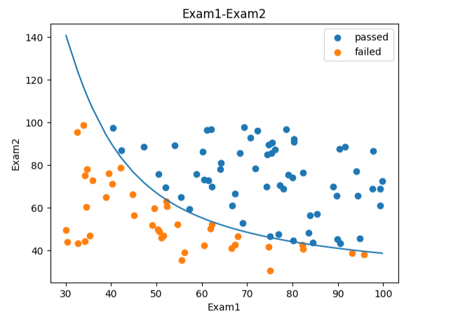

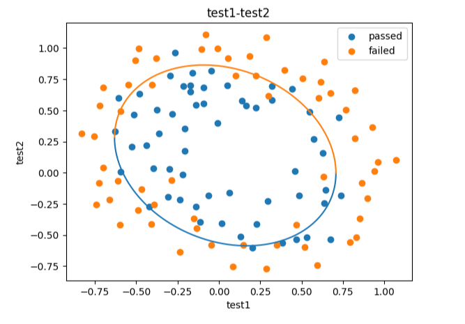
四、芯片质量预测实战，使用数据集chip_test.csv

复制代码

#加载数据
import pandas as pd
import numpy as np
data = pd.read_csv('chip_test.csv')
data.head()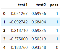

复制代码

#画散点图
from matplotlib import pyplot as plt
fig6 = plt.figure()
plt.scatter(data.loc[:,'test1'],data.loc[:,'test2'])
plt.title("test1-test2")
plt.xlabel("test1")
plt.ylabel("test2")
plt.show()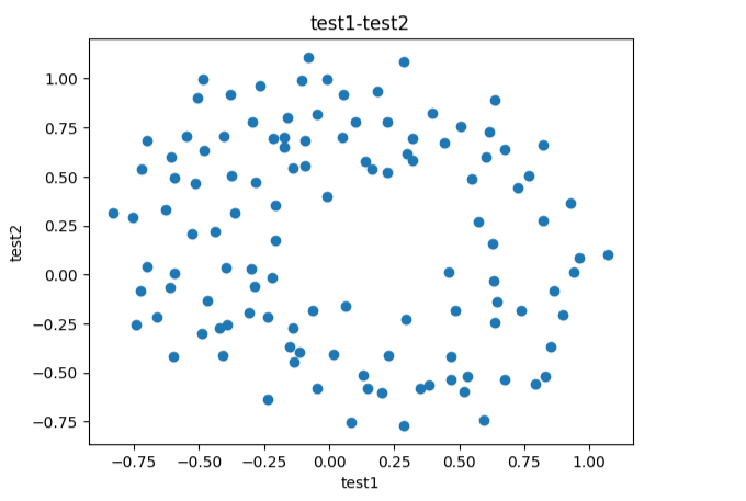

复制代码

#区分数据
mask = data.loc[:,'pass']==1
print(mask)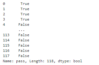

复制代码

fig7 = plt.figure()
passed = plt.scatter(data.loc[:,'test1'][mask],data.loc[:,'test2'][mask])
failed = plt.scatter(data.loc[:,'test1'][~mask],data.loc[:,'test2'][~mask])
plt.title("test1-test2")
plt.xlabel("test1")
plt.ylabel("test2")
plt.legend((passed,failed),("passed","failed"))
plt.show()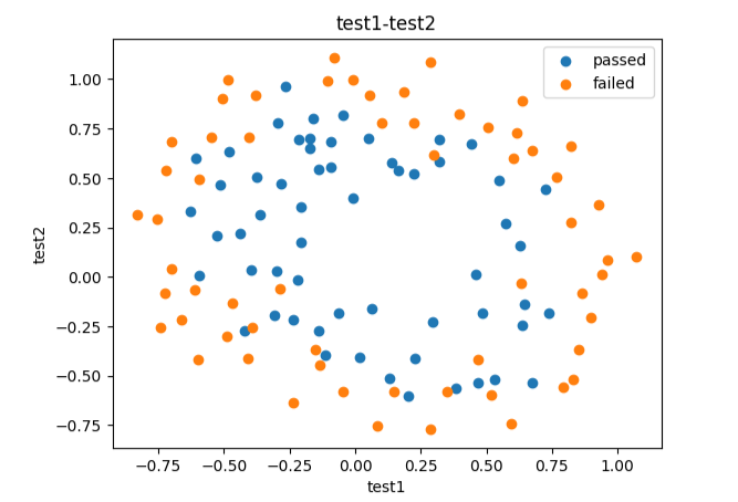

复制代码

#赋值x，y
x = data.drop(['pass'],axis=1)
x1 = data.loc[:,'test1']
x2 = data.loc[:,'test2']
y = data.loc[:,'pass']
#使用二阶边界函数
X1_2 = x1*x1
X2_2 = x2*x2
X1_X2 = x1*x2

X_new = {'X1':x1,'X2':x2,'X1_2':X1_2,'X2_2':X2_2,'X1_X2':X1_X2}
X_new = pd.DataFrame(X_new)
print(X_new)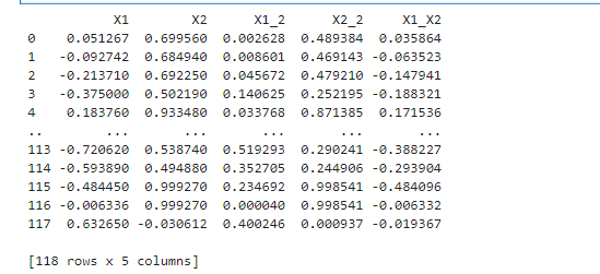

复制代码

#创建模型2
LR2 = LogisticRegression(solver='liblinear', max_iter=1000)# solver='saga',    # 最通用的求解器 max_iter=1000,    # 足够的迭代次数
LR2.fit(X_new,y)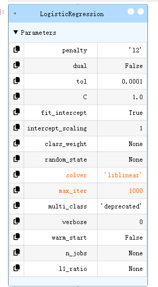

复制代码

#预测结果
y_2_predict = LR2.predict(X_new)
print(y_2_predict)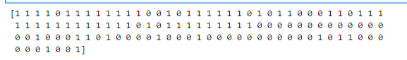

复制代码

#打印预测准确率
accuracy = accuracy_score(y,y_2_predict)
print(accuracy)

复制代码

#对x1排序
X1_new = x1.sort_values()
print(x1,X1_new)

LR2.coef_

theta0 = LR2.intercept_
theta1,theta2,theta3,theta4,theta5 = LR2.coef_[0][0],LR2.coef_[0][1],LR2.coef_[0][2],LR2.coef_[0][3],LR2.coef_[0][4]

print(theta0,theta1,theta2,theta3,theta4,theta5)

复制代码

a = theta4
b = theta5*X1_new+theta2
c = theta0+theta1*X1_new+theta3*X1_new*X1_new
X2_new_boundary = (-b+np.sqrt(b*b-4*a*c))/(2*a)
print(X2_new_boundary)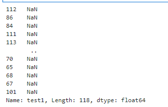

复制代码

fig8 = plt.figure()
plt.plot(X1_new,X2_new_boundary)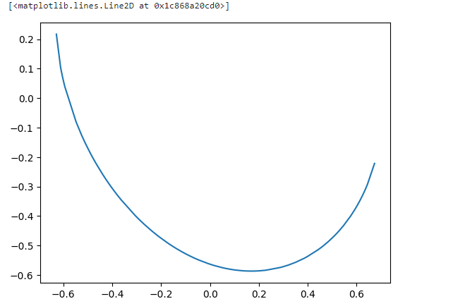

复制代码

fig9 = plt.figure()
passed = plt.scatter(data.loc[:,'test1'][mask],data.loc[:,'test2'][mask])
failed = plt.scatter(data.loc[:,'test1'][~mask],data.loc[:,'test2'][~mask])
plt.plot(X1_new,X2_new_boundary)
plt.title("test1-test2")
plt.xlabel("test1")
plt.ylabel("test2")
plt.legend((passed,failed),("passed","failed"))
plt.show()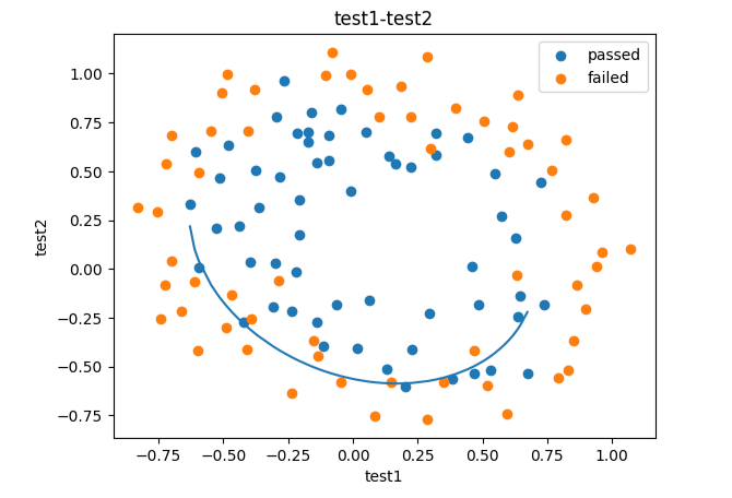

复制代码

#定义边界函数
def f(x):
    a = theta4
    b = theta5*x+theta2
    c = theta0+theta1*x+theta3*x*x
    X2_new_boundary1 = (-b+np.sqrt(b*b-4*a*c))/(2*a)
    X2_new_boundary2 = (-b-np.sqrt(b*b-4*a*c))/(2*a)
    return X2_new_boundary1,X2_new_boundary2

X2_new_boundary1 = []
X2_new_boundary2 = []
for x in X1_new:
    X2_new_boundary1.append(f(x)[0])
    X2_new_boundary2.append(f(x)[1])
print(X2_new_boundary1,X2_new_boundary2)

fig10 = plt.figure()
passed = plt.scatter(data.loc[:,'test1'][mask],data.loc[:,'test2'][mask])
failed = plt.scatter(data.loc[:,'test1'][~mask],data.loc[:,'test2'][~mask])
plt.plot(X1_new,X2_new_boundary1)
plt.plot(X1_new,X2_new_boundary2)
plt.title("test1-test2")
plt.xlabel("test1")
plt.ylabel("test2")
plt.legend((passed,failed),("passed","failed"))
plt.show()

复制代码

X1_range = [-0.9+x/10000 for x in range(0,19000)]
X1_range = np.array(X1_range)
X2_new_boundary1 = []
X2_new_boundary2 = []
for x in X1_range:
    X2_new_boundary1.append(f(x)[0])
    X2_new_boundary2.append(f(x)[1])
print(X2_new_boundary1,X2_new_boundary2)

fig11 = plt.figure()
passed = plt.scatter(data.loc[:,'test1'][mask],data.loc[:,'test2'][mask])
failed = plt.scatter(data.loc[:,'test1'][~mask],data.loc[:,'test2'][~mask])
plt.plot(X1_range,X2_new_boundary1)
plt.plot(X1_range,X2_new_boundary2)
plt.title("test1-test2")
plt.xlabel("test1")
plt.ylabel("test2")
plt.legend((passed,failed),("passed","failed"))
plt.show()