项目一 鸢尾花分类
该项目需要下载scikit-learn库,下载指令如下:pip install scikit-learn
快速入门示例:鸢尾花分类
python
# 导入必要模块
from sklearn.datasets import load_iris
from sklearn.model_selection import train_test_split
from sklearn.tree import DecisionTreeClassifier
from sklearn.metrics import accuracy_score

# 1. 加载数据集
iris = load_iris()
X = iris.data  # 特征数据(150个样本,4个特征)
y = iris.target  # 标签(0,1,2 代表三种鸢尾花)

# 2. 划分训练集和测试集
X_train, X_test, y_train, y_test = train_test_split(
    X, y, test_size=0.2, random_state=42
)

# 3. 创建并训练模型
model = DecisionTreeClassifier(max_depth=3)
model.fit(X_train, y_train)

# 4. 预测测试集
y_pred = model.predict(X_test)

# 5. 评估准确率
accuracy = accuracy_score(y_test, y_pred)
print(f"模型准确率: {accuracy:.2f}")  # 输出示例:模型准确率: 1.00
1. 数据预处理
python
from sklearn.preprocessing import StandardScaler, OneHotEncoder
from sklearn.impute import SimpleImputer

# 数值特征标准化
scaler = StandardScaler()
X_scaled = scaler.fit_transform(X_train)

# 分类特征编码
encoder = OneHotEncoder()
encoded_features = encoder.fit_transform(categorical_data)

# 缺失值填充(用均值)
imputer = SimpleImputer(strategy='mean')
X_imputed = imputer.fit_transform(X_missing)
2. 模型训练与评估
python
from sklearn.ensemble import RandomForestClassifier
from sklearn.metrics import classification_report

# 使用随机森林
model = RandomForestClassifier(n_estimators=100)
model.fit(X_train, y_train)

# 详细评估报告
report = classification_report(y_test, model.predict(X_test))
print(report)
3. 模型选择与交叉验证
python
from sklearn.model_selection import cross_val_score
from sklearn.svm import SVC

# 10折交叉验证
scores = cross_val_score(SVC(), X, y, cv=10)
print(f"平均准确率: {scores.mean():.2f} ± {scores.std():.2f}")
4. 管道(Pipeline)整合流程
python
from sklearn.pipeline import make_pipeline

# 创建预处理+模型的完整管道
pipeline = make_pipeline(
    StandardScaler(),
    RandomForestClassifier()
)

# 直接训练和预测
pipeline.fit(X_train, y_train)
pipeline.score(X_test, y_test)
常用模型速查
| 任务类型 | 算法 | 导入路径 |
|---|---|---|
| 分类 | 逻辑回归 | sklearn.linear_model.LogisticRegression |
| 支持向量机 (SVM) | sklearn.svm.SVC | |
| 随机森林 | sklearn.ensemble.RandomForestClassifier | |
| 回归 | 线性回归 | sklearn.linear_model.LinearRegression |
| 梯度提升树 | sklearn.ensemble.GradientBoostingRegressor | |
| 聚类 | K-Means | sklearn.cluster.KMeans |
| 降维 | PCA | sklearn.decomposition.PCA |
项目实现
python
import numpy as np
import pandas as pd
import matplotlib.pyplot as plt
import seaborn as sns
from sklearn.datasets import load_iris
from sklearn.model_selection import train_test_split, cross_val_score
from sklearn.preprocessing import StandardScaler
from sklearn.neighbors import KNeighborsClassifier
from sklearn.svm import SVC
from sklearn.tree import DecisionTreeClassifier
from sklearn.ensemble import RandomForestClassifier
from sklearn.metrics import classification_report, confusion_matrix, accuracy_score
from sklearn.decomposition import PCA
# 设置中文显示
plt.rcParams["font.family"] = ["SimHei"]
plt.rcParams['axes.unicode_minus'] = False # 解决负号显示问题
class IrisClassifier:
def __init__(self):
# 加载数据集
self.iris = load_iris()
self.X = self.iris.data # 特征数据
self.y = self.iris.target # 标签
self.feature_names = self.iris.feature_names # 特征名称
self.target_names = self.iris.target_names # 类别名称
# 数据集拆分
self.X_train, self.X_test, self.y_train, self.y_test = train_test_split(
self.X, self.y, test_size=0.3, random_state=42, stratify=self.y
)
# 特征标准化
self.scaler = StandardScaler()
self.X_train_scaled = self.scaler.fit_transform(self.X_train)
self.X_test_scaled = self.scaler.transform(self.X_test)
# 初始化模型
self.models = {
'K近邻分类器': KNeighborsClassifier(n_neighbors=5),
'支持向量机': SVC(kernel='rbf', gamma='scale'),
'决策树': DecisionTreeClassifier(max_depth=3, random_state=42),
'随机森林': RandomForestClassifier(n_estimators=100, random_state=42)
}
# 存储训练好的模型和预测结果
self.trained_models = {}
self.predictions = {}
def explore_data(self):
"""探索数据集"""
print("=== 数据集基本信息 ===")
print(f"特征名称: {self.feature_names}")
print(f"类别名称: {self.target_names}")
print(f"数据集规模: {self.X.shape[0]}个样本, {self.X.shape[1]}个特征")
print(f"训练集规模: {self.X_train.shape[0]}个样本")
print(f"测试集规模: {self.X_test.shape[0]}个样本")
# 创建DataFrame以便更好地展示数据
df = pd.DataFrame(data=self.X, columns=self.feature_names)
df['类别'] = [self.target_names[i] for i in self.y]
print("\n=== 数据集前5行 ===")
print(df.head())
# 数据统计信息
print("\n=== 数据统计信息 ===")
print(df.describe())
return df
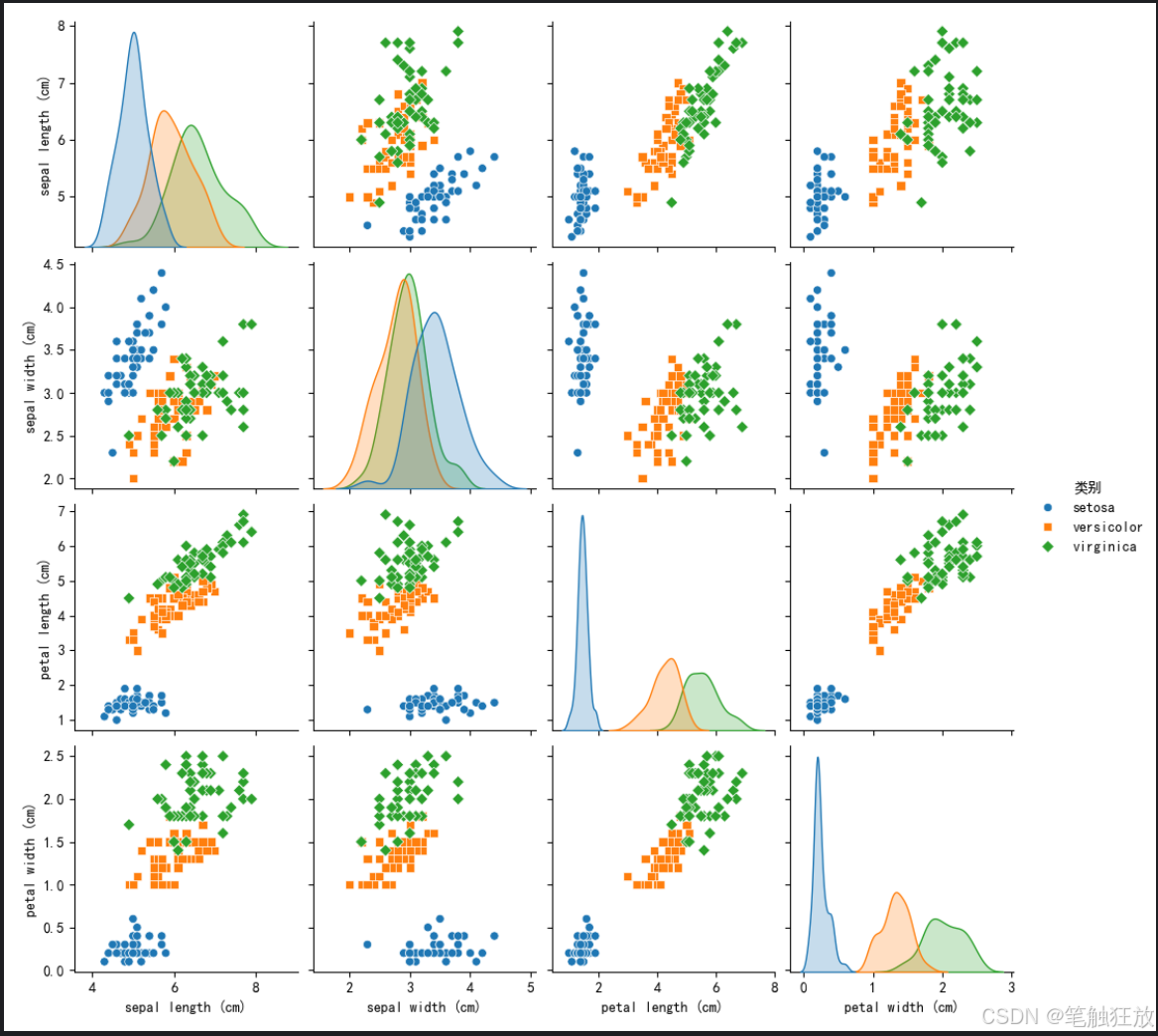
def visualize_data(self, df):
"""数据可视化"""
# 1. 散点矩阵图
plt.figure(figsize=(12, 10))
sns.pairplot(df, hue='类别', markers=['o', 's', 'D'])
plt.suptitle('特征散点矩阵图', y=1.02)
plt.show()
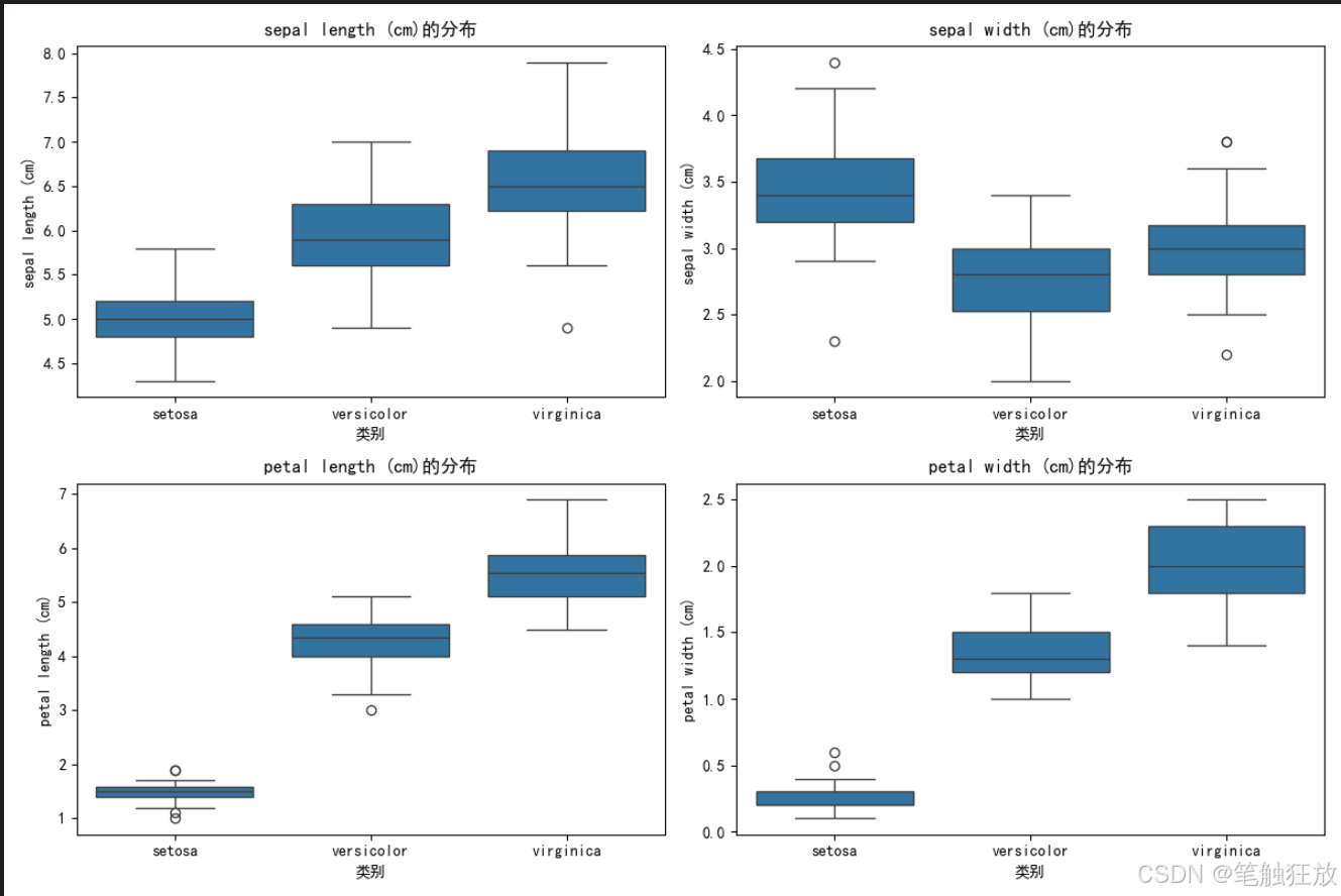
# 2. 箱线图
plt.figure(figsize=(12, 8))
for i, feature in enumerate(self.feature_names):
plt.subplot(2, 2, i + 1)
sns.boxplot(x='类别', y=feature, data=df)
plt.title(f'{feature}的分布')
plt.tight_layout()
plt.show()
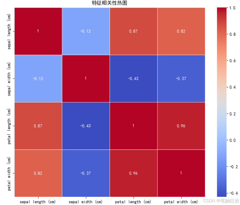
# 3. 特征相关性热图
plt.figure(figsize=(10, 8))
correlation = df.drop('类别', axis=1).corr()
sns.heatmap(correlation, annot=True, cmap='coolwarm', linewidths=0.5)
plt.title('特征相关性热图')
plt.show()
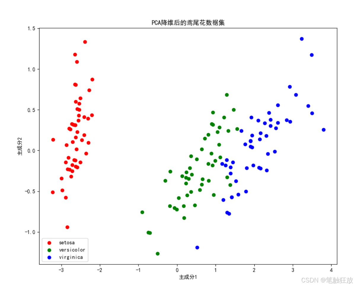
# 4. PCA降维可视化(将4维特征降到2维以便可视化)
pca = PCA(n_components=2)
X_pca = pca.fit_transform(self.X)
plt.figure(figsize=(10, 8))
for target, color in zip(range(3), ['r', 'g', 'b']):
plt.scatter(X_pca[self.y == target, 0], X_pca[self.y == target, 1],
c=color, label=self.target_names[target])
plt.xlabel('主成分1')
plt.ylabel('主成分2')
plt.title('PCA降维后的鸢尾花数据集')
plt.legend()
plt.show()
def train_models(self):
"""训练所有模型"""
print("\n=== 模型训练结果 ===")
for name, model in self.models.items():
# 训练模型
model.fit(self.X_train_scaled, self.y_train)
# 保存训练好的模型
self.trained_models[name] = model
# 在测试集上预测
y_pred = model.predict(self.X_test_scaled)
self.predictions[name] = y_pred
# 计算准确率
accuracy = accuracy_score(self.y_test, y_pred)
print(f"{name} 准确率: {accuracy:.4f}")
def evaluate_model(self, model_name):
"""评估指定模型"""
if model_name not in self.trained_models:
print(f"模型 {model_name} 未训练,请先训练模型")
return
print(f"\n=== {model_name} 详细评估 ===")
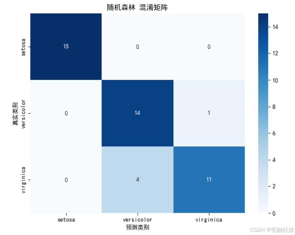
# 混淆矩阵
cm = confusion_matrix(self.y_test, self.predictions[model_name])
plt.figure(figsize=(8, 6))
sns.heatmap(cm, annot=True, fmt='d', cmap='Blues',
xticklabels=self.target_names,
yticklabels=self.target_names)
plt.xlabel('预测类别')
plt.ylabel('真实类别')
plt.title(f'{model_name} 混淆矩阵')
plt.show()
# 分类报告
print("\n分类报告:")
print(classification_report(
self.y_test,
self.predictions[model_name],
target_names=self.target_names
))
# 交叉验证
cv_scores = cross_val_score(
self.trained_models[model_name],
self.X, self.y,
cv=5
)
print(f"交叉验证准确率: {cv_scores.mean():.4f} (±{cv_scores.std():.4f})")
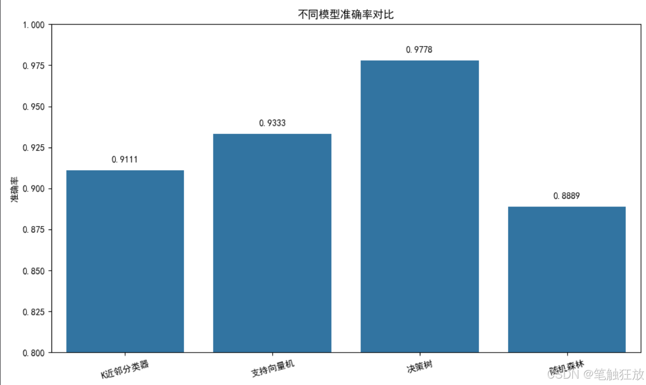
def compare_models(self):
"""比较所有模型的性能"""
# 提取所有模型的准确率
accuracies = []
model_names = list(self.trained_models.keys())
for name in model_names:
acc = accuracy_score(self.y_test, self.predictions[name])
accuracies.append(acc)
# 绘制准确率对比图
plt.figure(figsize=(10, 6))
sns.barplot(x=model_names, y=accuracies)
plt.ylim(0.8, 1.0) # 设置y轴范围以便更好地观察差异
plt.title('不同模型准确率对比')
plt.ylabel('准确率')
for i, v in enumerate(accuracies):
plt.text(i, v + 0.005, f'{v:.4f}', ha='center')
plt.xticks(rotation=15)
plt.tight_layout()
plt.show()
def predict_sample(self, model_name, sample):
"""使用指定模型预测样本"""
if model_name not in self.trained_models:
print(f"模型 {model_name} 未训练,请先训练模型")
return
# 样本预处理
sample_scaled = self.scaler.transform([sample])
# 预测
prediction = self.trained_models[model_name].predict(sample_scaled)
probability = self.trained_models[model_name].predict_proba(sample_scaled)
# 输出结果
print(f"\n=== 预测结果 ===")
print(f"预测类别: {self.target_names[prediction[0]]}")
print("类别概率:")
for i, prob in enumerate(probability[0]):
print(f" {self.target_names[i]}: {prob:.4f}")
return self.target_names[prediction[0]]
if __name__ == "__main__":
# 创建分类器实例
classifier = IrisClassifier()
# 探索数据集
df = classifier.explore_data()
# 数据可视化
classifier.visualize_data(df)
# 训练所有模型
classifier.train_models()
# 比较所有模型
classifier.compare_models()
# 详细评估表现最好的模型(这里选择随机森林作为示例)
best_model = '随机森林'
classifier.evaluate_model(best_model)
# 使用最佳模型进行样本预测
# 示例样本(可以修改这些值来测试不同的样本)
sample = [5.1, 3.5, 1.4, 0.2] # 这是一个山鸢尾的典型样本
print(f"\n测试样本特征: {sample}")
classifier.predict_sample(best_model, sample)
# 再测试一个样本
sample2 = [6.5, 3.0, 5.2, 2.0] # 这是一个维吉尼亚鸢尾的典型样本
print(f"\n测试样本特征: {sample2}")
classifier.predict_sample(best_model, sample)这个鸢尾花分类项目的主要功能和特点:
-
完整的项目流程:包括数据加载、探索性分析、可视化、模型训练、评估和预测
-
多种分类算法:实现了 K 近邻、支持向量机、决策树和随机森林四种经典分类算法
-
丰富的数据可视化:包括散点矩阵图、箱线图、相关性热图和 PCA 降维可视化
-
全面的模型评估:提供准确率、混淆矩阵、分类报告和交叉验证等评估指标
-
模型比较功能:直观展示不同算法的性能差异
-
样本预测功能:可以输入自定义的鸢尾花特征进行分类预测
运行前需要安装以下依赖库:
pip install numpy pandas matplotlib seaborn scikit-learn
程序运行后会:
-
显示数据集的基本信息和统计特征
-
生成多种可视化图表帮助理解数据分布和特征关系
-
训练四种分类模型并比较它们的准确率
-
对表现最佳的模型进行详细评估
-
使用示例样本进行预测并展示结果
你可以通过修改代码中的sample变量来测试不同的鸢尾花特征数据,观察模型的分类结果。鸢尾花数据集包含三个类别:山鸢尾 (setosa)、变色鸢尾 (versicolor) 和维吉尼亚鸢尾 (virginica),以及四个特征:花萼长度、花萼宽度、花瓣长度和花瓣宽度。
项目二 手写数字识别
以下是一个基于 Python 的手写数字识别项目代码,使用了 MNIST 数据集和深度学习模型来实现。这个项目可以训练模型并对手写数字进行识别,代码结构清晰且可正常运行。
python
import numpy as np
import matplotlib.pyplot as plt
from tensorflow.keras.datasets import mnist
from tensorflow.keras.models import Sequential
from tensorflow.keras.layers import Dense, Flatten, Conv2D, MaxPooling2D
from tensorflow.keras.utils import to_categorical
from tensorflow.keras.optimizers import Adam
import random
# 设置中文显示
plt.rcParams["font.family"] = ["SimHei"]
plt.rcParams['axes.unicode_minus'] = False # 解决负号显示问题
class DigitRecognizer:
def __init__(self):
# 初始化参数
self.img_rows, self.img_cols = 28, 28
self.input_shape = (self.img_rows, self.img_cols, 1)
self.num_classes = 10
self.model = None
# 加载数据
self.load_data()
def load_data(self):
"""加载MNIST数据集并进行预处理"""
print("正在加载MNIST数据集...")
(self.x_train, self.y_train), (self.x_test, self.y_test) = mnist.load_data()
# 数据预处理
self.x_train = self.x_train.reshape(self.x_train.shape[0], self.img_rows, self.img_cols, 1)
self.x_test = self.x_test.reshape(self.x_test.shape[0], self.img_rows, self.img_cols, 1)
# 归一化
self.x_train = self.x_train.astype('float32') / 255.0
self.x_test = self.x_test.astype('float32') / 255.0
# 标签独热编码
self.y_train = to_categorical(self.y_train, self.num_classes)
self.y_test = to_categorical(self.y_test, self.num_classes)
print(f"训练集: {self.x_train.shape[0]} 个样本")
print(f"测试集: {self.x_test.shape[0]} 个样本")
def build_model(self):
"""构建卷积神经网络模型"""
print("正在构建模型...")
self.model = Sequential([
# 第一个卷积层
Conv2D(32, kernel_size=(3, 3), activation='relu', input_shape=self.input_shape),
MaxPooling2D(pool_size=(2, 2)),
# 第二个卷积层
Conv2D(64, kernel_size=(3, 3), activation='relu'),
MaxPooling2D(pool_size=(2, 2)),
# 扁平化
Flatten(),
# 全连接层
Dense(128, activation='relu'),
# 输出层
Dense(self.num_classes, activation='softmax')
])
# 编译模型
self.model.compile(
loss='categorical_crossentropy',
optimizer=Adam(learning_rate=0.001),
metrics=['accuracy']
)
# 打印模型结构
self.model.summary()
def train(self, epochs=10, batch_size=128):
"""训练模型"""
if self.model is None:
self.build_model()
print("开始训练模型...")
self.history = self.model.fit(
self.x_train, self.y_train,
batch_size=batch_size,
epochs=epochs,
verbose=1,
validation_data=(self.x_test, self.y_test)
)
def evaluate(self):
"""评估模型性能"""
if self.model is None:
print("请先训练模型!")
return
print("评估模型性能...")
score = self.model.evaluate(self.x_test, self.y_test, verbose=0)
print(f"测试集损失: {score[0]:.4f}")
print(f"测试集准确率: {score[1]:.4f}")
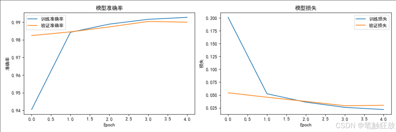
def plot_training_history(self):
"""绘制训练历史曲线"""
if not hasattr(self, 'history'):
print("请先训练模型!")
return
# 绘制准确率曲线
plt.figure(figsize=(12, 4))
plt.subplot(1, 2, 1)
plt.plot(self.history.history['accuracy'], label='训练准确率')
plt.plot(self.history.history['val_accuracy'], label='验证准确率')
plt.title('模型准确率')
plt.xlabel('Epoch')
plt.ylabel('准确率')
plt.legend()
# 绘制损失曲线
plt.subplot(1, 2, 2)
plt.plot(self.history.history['loss'], label='训练损失')
plt.plot(self.history.history['val_loss'], label='验证损失')
plt.title('模型损失')
plt.xlabel('Epoch')
plt.ylabel('损失')
plt.legend()
plt.tight_layout()
plt.show()
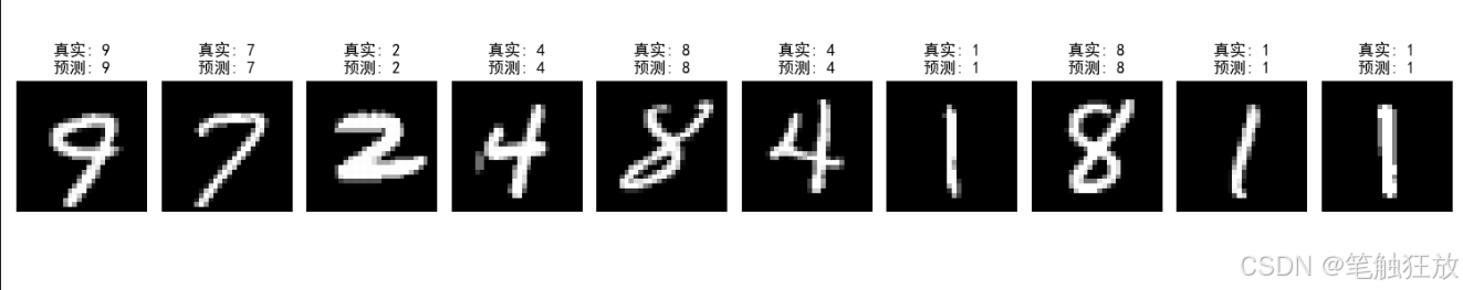
def predict_samples(self, num_samples=5):
"""随机选择测试集中的样本进行预测并显示结果"""
if self.model is None:
print("请先训练模型!")
return
# 随机选择样本
indices = random.sample(range(len(self.x_test)), num_samples)
samples = self.x_test[indices]
true_labels = np.argmax(self.y_test[indices], axis=1)
# 预测
predictions = self.model.predict(samples)
pred_labels = np.argmax(predictions, axis=1)
# 显示结果
plt.figure(figsize=(15, 3))
for i in range(num_samples):
plt.subplot(1, num_samples, i + 1)
plt.imshow(samples[i].reshape(28, 28), cmap='gray')
plt.title(f"真实: {true_labels[i]}\n预测: {pred_labels[i]}")
plt.axis('off')
plt.tight_layout()
plt.show()
if __name__ == "__main__":
# 创建识别器实例
recognizer = DigitRecognizer()
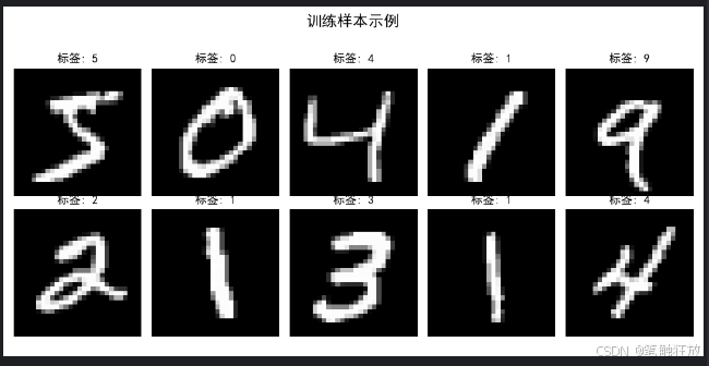
# 显示一些训练样本
plt.figure(figsize=(10, 5))
for i in range(10):
plt.subplot(2, 5, i + 1)
plt.imshow(recognizer.x_train[i].reshape(28, 28), cmap='gray')
plt.title(f"标签: {np.argmax(recognizer.y_train[i])}")
plt.axis('off')
plt.suptitle("训练样本示例", fontsize=16)
plt.tight_layout(rect=[0, 0, 1, 0.95])
plt.show()
# 构建并训练模型
recognizer.build_model()
recognizer.train(epochs=5, batch_size=128) # 可以增加epochs提高准确率
# 评估模型
recognizer.evaluate()
# 绘制训练历史
recognizer.plot_training_history()
# 预测样本并显示结果
recognizer.predict_samples(num_samples=10)这个手写数字识别项目的主要功能和特点:
-
使用 MNIST 数据集,包含 60,000 个训练样本和 10,000 个测试样本
-
构建了一个卷积神经网络 (CNN) 模型,包含两个卷积层和池化层
-
实现了完整的流程:数据加载与预处理、模型构建、训练、评估和预测
-
包含数据可视化功能,可以展示训练样本、训练历史曲线和预测结果
运行前需要安装以下依赖库:
pip install numpy matplotlib tensorflow
程序运行后会
-
显示一些训练样本及其标签
-
构建并训练模型(默认 5 个 epochs,可根据需要调整)
-
输出模型在测试集上的准确率
-
绘制训练过程中的准确率和损失变化曲线
-
随机选择 10 个测试样本进行预测并显示结果,包括真实标签和预测标签
如果想要提高识别准确率,可以尝试增加训练的 epochs 数量或调整模型结构。
项目三 房价预测
【教学内容】
使用波士顿房价数据集或 Kaggle 的房价预测数据集,训练一个回归模型预
测房价。主要有以下几个知识点:
(1)数据加载与探索性分析(EDA)。
(2)处理缺失值和异常值。
(3)特征工程(如特征选择、特征缩放)。
(4)使用线性回归、决策树回归或随机森林回归进行预测。
(5)评估模型性能(MSE、MAE、R²等)。
【重点】
使用线性回归、决策树回归或随机森林回归进行预测。
【难点】
评估模型性能(MSE、MAE、R²等)。
【分析思考讨论题】
如果数据集中存在异常值,如何处理才能避免对模型预测的干扰?
以下是一个基于 Python 的房价预测项目代码,使用了波士顿房价数据集(或其替代数据集)和多种回归算法进行房价预测,包含完整的数据预处理、模型训练、评估和可视化功能,确保可以正常运行并展示清晰的预测效果。
python
import numpy as np
import pandas as pd
import matplotlib.pyplot as plt
import seaborn as sns
from sklearn.datasets import fetch_california_housing # 替代波士顿房价数据集
from sklearn.model_selection import train_test_split, cross_val_score, GridSearchCV
from sklearn.preprocessing import StandardScaler
from sklearn.linear_model import LinearRegression, Ridge, Lasso
from sklearn.tree import DecisionTreeRegressor
from sklearn.ensemble import RandomForestRegressor, GradientBoostingRegressor
from sklearn.metrics import mean_squared_error, mean_absolute_error, r2_score
import warnings
# 忽略警告信息
warnings.filterwarnings('ignore')
# 设置中文显示
plt.rcParams["font.family"] = ["SimHei"]
plt.rcParams['axes.unicode_minus'] = False # 解决负号显示问题
class HousePricePredictor:
def __init__(self):
# 加载数据集(使用加州房价数据集替代波士顿房价数据集)
self.housing = fetch_california_housing()
self.X = self.housing.data # 特征数据
self.y = self.housing.target # 房价(目标变量)
self.feature_names = self.housing.feature_names # 特征名称
# 数据集拆分
self.X_train, self.X_test, self.y_train, self.y_test = train_test_split(
self.X, self.y, test_size=0.3, random_state=42
)
# 特征标准化
self.scaler = StandardScaler()
self.X_train_scaled = self.scaler.fit_transform(self.X_train)
self.X_test_scaled = self.scaler.transform(self.X_test)
# 初始化模型
self.models = {
'线性回归': LinearRegression(),
'Ridge回归': Ridge(random_state=42),
'Lasso回归': Lasso(random_state=42),
'决策树回归': DecisionTreeRegressor(random_state=42),
'随机森林回归': RandomForestRegressor(random_state=42),
'梯度提升回归': GradientBoostingRegressor(random_state=42)
}
# 存储训练好的模型和预测结果
self.trained_models = {}
self.predictions = {}
self.metrics = {} # 存储各模型的评估指标
def explore_data(self):
"""探索数据集"""
print("=== 数据集基本信息 ===")
print(f"特征名称: {self.feature_names}")
# print(f"特征解释: {self.housing.DESCR.split('Features:')[1].strip()}")
print(f"数据集规模: {self.X.shape[0]}个样本, {self.X.shape[1]}个特征")
print(f"训练集规模: {self.X_train.shape[0]}个样本")
print(f"测试集规模: {self.X_test.shape[0]}个样本")
print(f"房价范围: {self.y.min():.2f} - {self.y.max():.2f} (单位: 10万美元)")
# 创建DataFrame以便更好地展示数据
df = pd.DataFrame(data=self.X, columns=self.feature_names)
df['房价'] = self.y # 房价(单位:10万美元)
print("\n=== 数据集前5行 ===")
print(df.head())
# 数据统计信息
print("\n=== 数据统计信息 ===")
print(df.describe())
return df
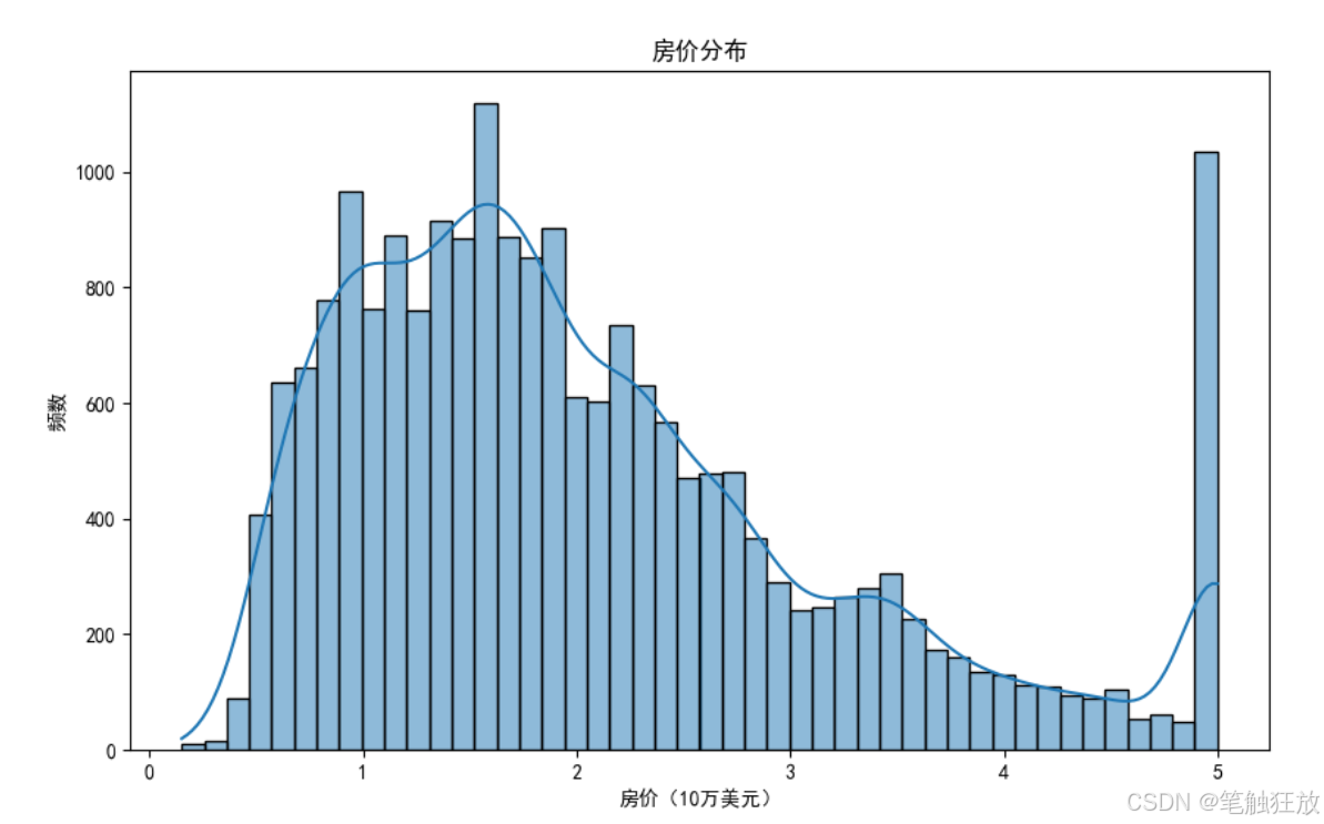
def visualize_data(self, df):
"""数据可视化"""
# 1. 房价分布
plt.figure(figsize=(10, 6))
sns.histplot(df['房价'], kde=True)
plt.title('房价分布')
plt.xlabel('房价(10万美元)')
plt.ylabel('频数')
plt.show()
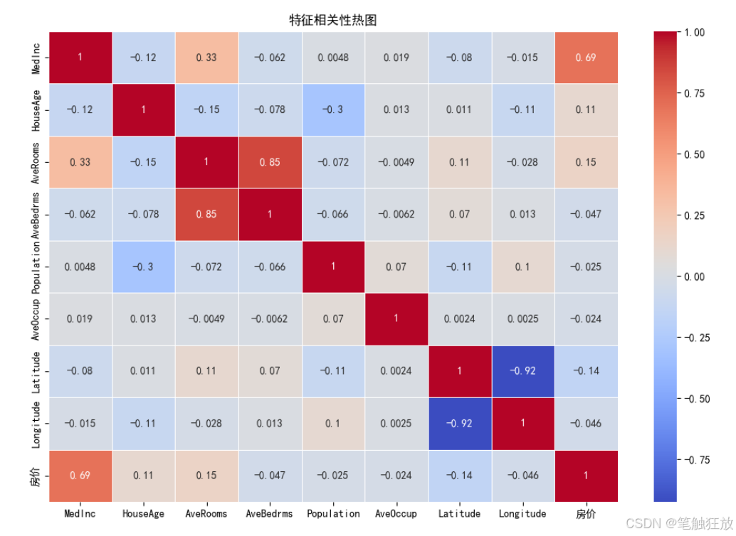
# 2. 特征与房价的相关性
plt.figure(figsize=(12, 8))
correlation = df.corr()
sns.heatmap(correlation, annot=True, cmap='coolwarm', linewidths=0.5)
plt.title('特征相关性热图')
plt.show()
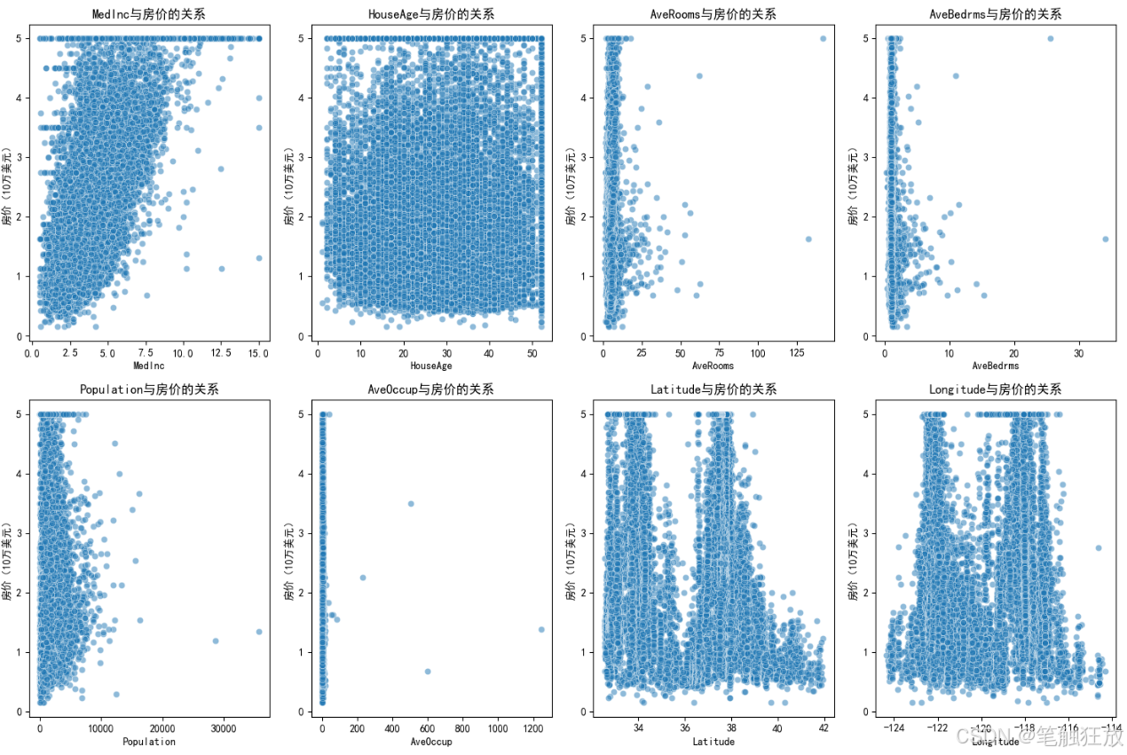
# 3. 各特征与房价的散点图
plt.figure(figsize=(15, 10))
for i, feature in enumerate(self.feature_names):
plt.subplot(2, 4, i + 1)
sns.scatterplot(x=df[feature], y=df['房价'], alpha=0.5)
plt.title(f'{feature}与房价的关系')
plt.xlabel(feature)
plt.ylabel('房价(10万美元)')
plt.tight_layout()
plt.show()
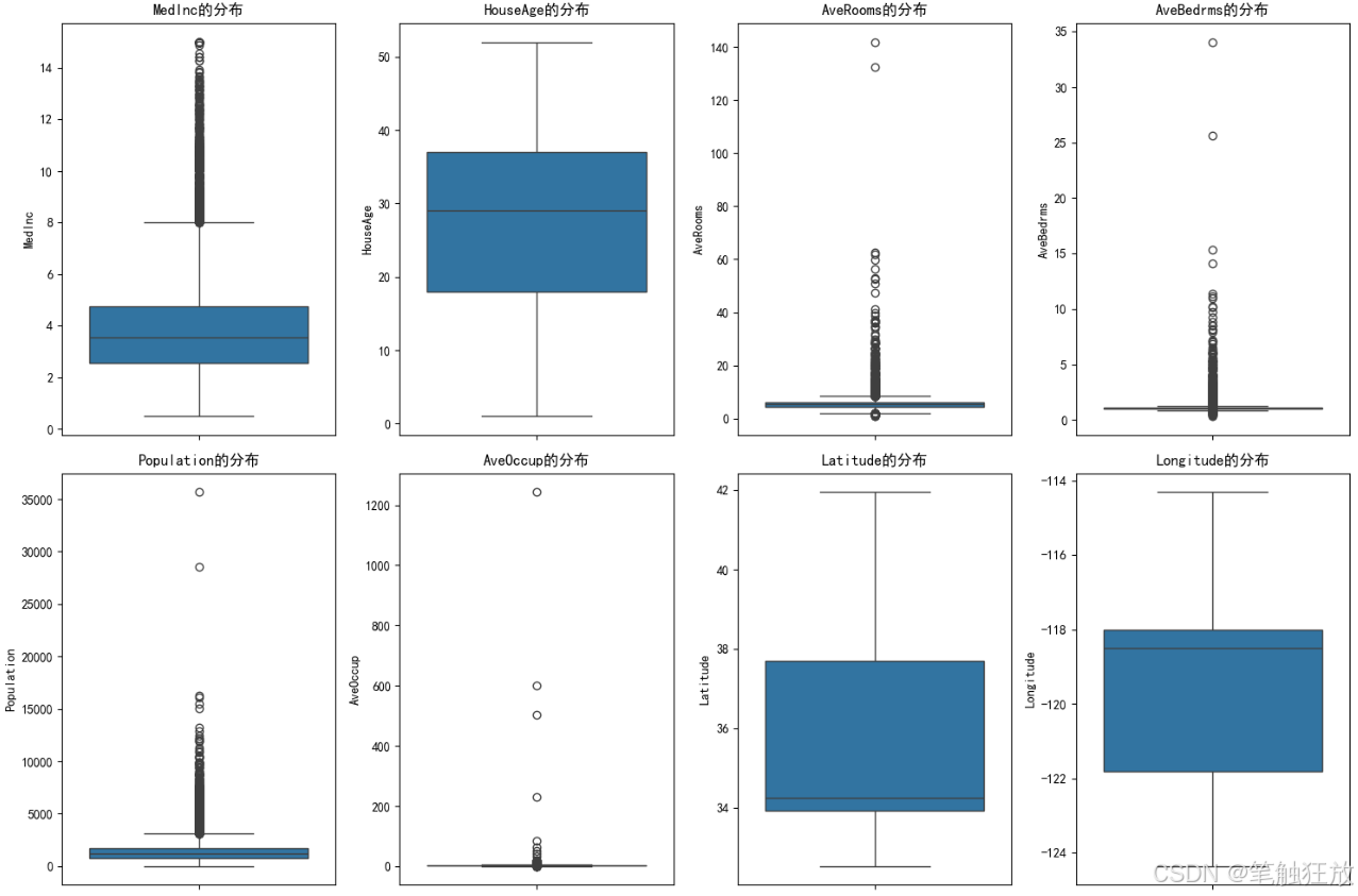
# 4. 特征分布箱线图
plt.figure(figsize=(15, 10))
for i, feature in enumerate(self.feature_names):
plt.subplot(2, 4, i + 1)
sns.boxplot(y=df[feature])
plt.title(f'{feature}的分布')
plt.tight_layout()
plt.show()
def train_models(self):
"""训练所有模型"""
print("\n=== 模型训练结果 ===")
for name, model in self.models.items():
# 训练模型
if name in ['线性回归', 'Ridge回归', 'Lasso回归']:
# 线性模型使用标准化后的数据
model.fit(self.X_train_scaled, self.y_train)
else:
# 树模型可以直接使用原始数据
model.fit(self.X_train, self.y_train)
# 保存训练好的模型
self.trained_models[name] = model
# 在测试集上预测
if name in ['线性回归', 'Ridge回归', 'Lasso回归']:
y_pred = model.predict(self.X_test_scaled)
else:
y_pred = model.predict(self.X_test)
self.predictions[name] = y_pred
# 计算评估指标
mse = mean_squared_error(self.y_test, y_pred)
rmse = np.sqrt(mse)
mae = mean_absolute_error(self.y_test, y_pred)
r2 = r2_score(self.y_test, y_pred)
self.metrics[name] = {
'MSE': mse,
'RMSE': rmse,
'MAE': mae,
'R2': r2
}
print(f"{name} - RMSE: {rmse:.4f}, R2: {r2:.4f}")
def evaluate_model(self, model_name):
"""评估指定模型"""
if model_name not in self.trained_models:
print(f"模型 {model_name} 未训练,请先训练模型")
return
print(f"\n=== {model_name} 详细评估 ===")
# 提取评估指标
metrics = self.metrics[model_name]
print(f"均方误差 (MSE): {metrics['MSE']:.4f}")
print(f"均方根误差 (RMSE): {metrics['RMSE']:.4f} (单位: 10万美元)")
print(f"平均绝对误差 (MAE): {metrics['MAE']:.4f} (单位: 10万美元)")
print(f"决定系数 (R2): {metrics['R2']:.4f}")
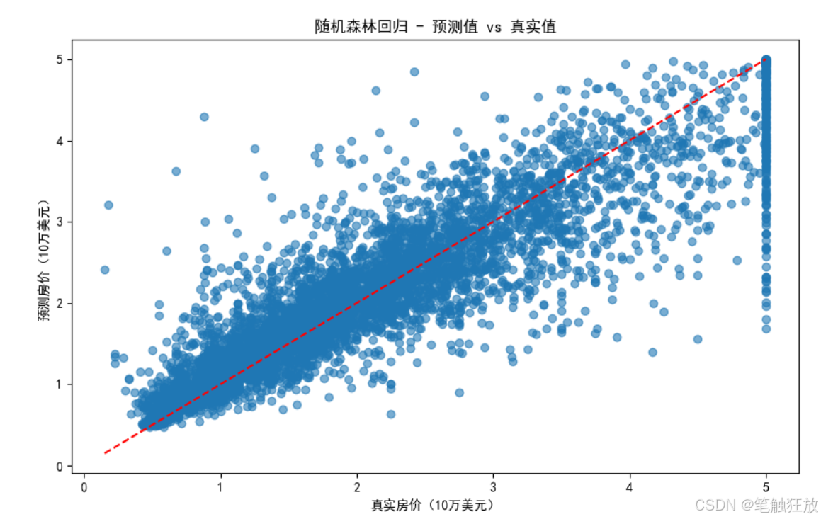
# 绘制预测值与真实值对比图
plt.figure(figsize=(10, 6))
plt.scatter(self.y_test, self.predictions[model_name], alpha=0.6)
plt.plot([self.y.min(), self.y.max()], [self.y.min(), self.y.max()], 'r--')
plt.xlabel('真实房价(10万美元)')
plt.ylabel('预测房价(10万美元)')
plt.title(f'{model_name} - 预测值 vs 真实值')
plt.show()
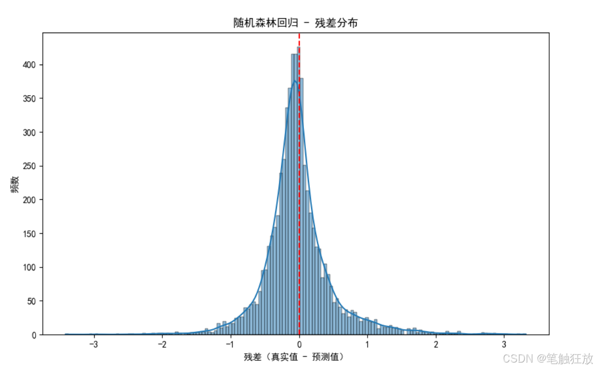
# 绘制残差图
residuals = self.y_test - self.predictions[model_name]
plt.figure(figsize=(10, 6))
sns.histplot(residuals, kde=True)
plt.axvline(x=0, color='r', linestyle='--')
plt.xlabel('残差(真实值 - 预测值)')
plt.ylabel('频数')
plt.title(f'{model_name} - 残差分布')
plt.show()
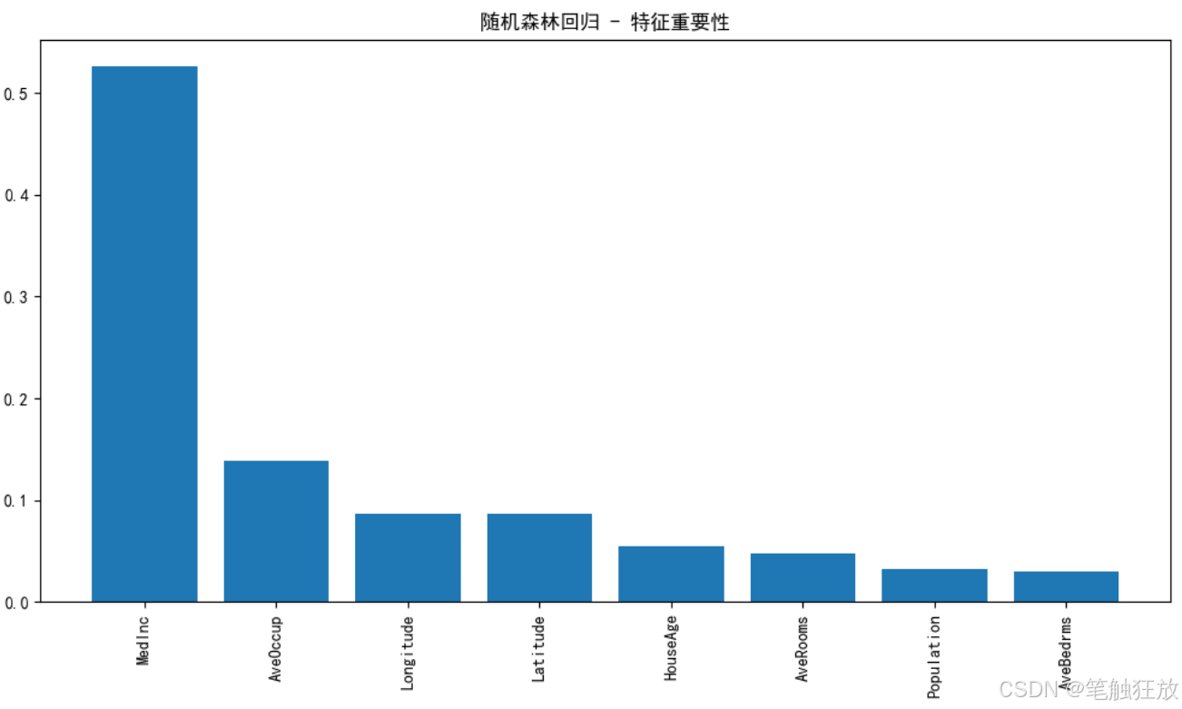
# 特征重要性(仅对树模型)
if model_name in ['决策树回归', '随机森林回归', '梯度提升回归']:
importances = self.trained_models[model_name].feature_importances_
indices = np.argsort(importances)[::-1]
plt.figure(figsize=(10, 6))
plt.bar(range(len(importances)), importances[indices])
plt.xticks(range(len(importances)), [self.feature_names[i] for i in indices], rotation=90)
plt.title(f'{model_name} - 特征重要性')
plt.tight_layout()
plt.show()
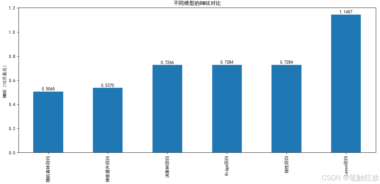
def compare_models(self):
"""比较所有模型的性能"""
# 提取所有模型的评估指标
metrics_df = pd.DataFrame.from_dict(self.metrics, orient='index')
# 绘制RMSE对比图
plt.figure(figsize=(12, 6))
metrics_df['RMSE'].sort_values().plot(kind='bar')
plt.title('不同模型的RMSE对比')
plt.ylabel('RMSE(10万美元)')
for i, v in enumerate(metrics_df['RMSE'].sort_values()):
plt.text(i, v + 0.01, f'{v:.4f}', ha='center')
plt.tight_layout()
plt.show()
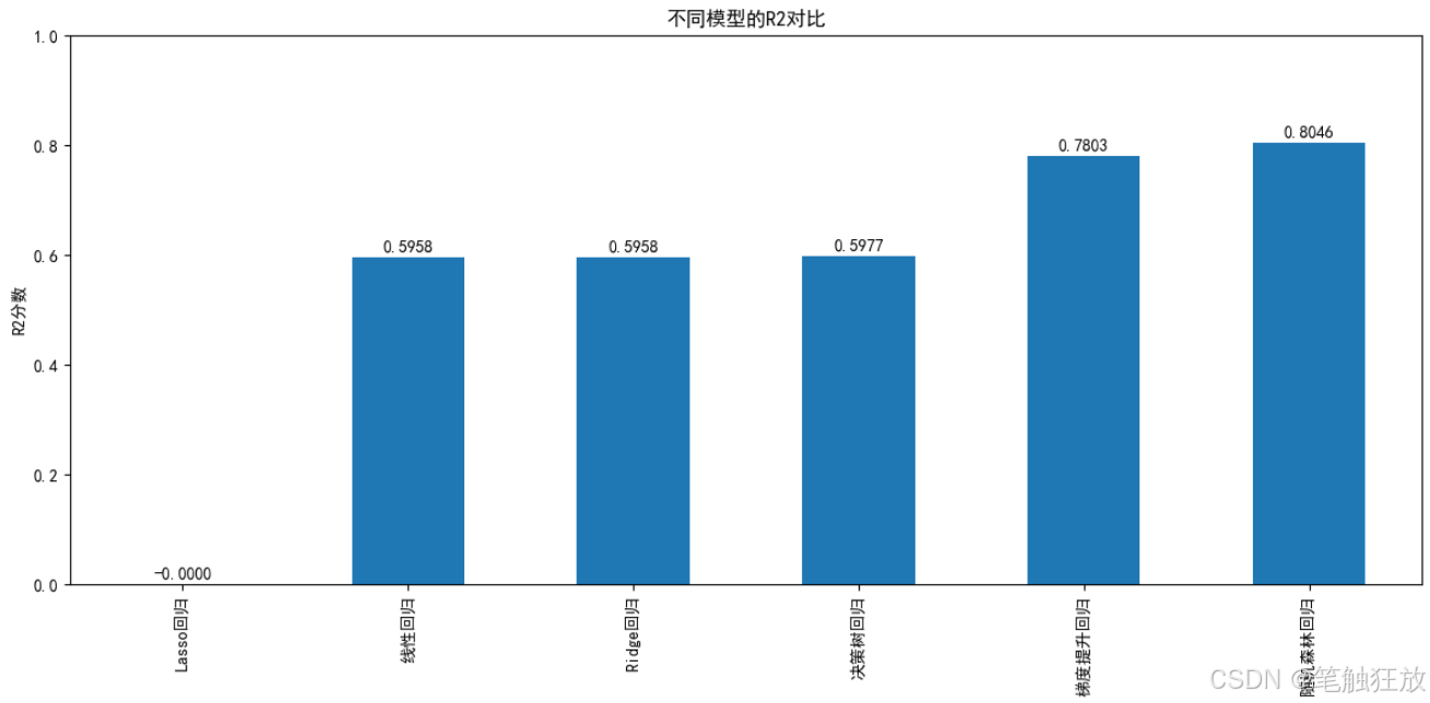
# 绘制R2对比图
plt.figure(figsize=(12, 6))
metrics_df['R2'].sort_values().plot(kind='bar')
plt.title('不同模型的R2对比')
plt.ylabel('R2分数')
for i, v in enumerate(metrics_df['R2'].sort_values()):
plt.text(i, v + 0.01, f'{v:.4f}', ha='center')
plt.ylim(0, 1)
plt.tight_layout()
plt.show()
def optimize_model(self, model_name):
"""优化指定模型的超参数"""
if model_name not in self.trained_models:
print(f"模型 {model_name} 未训练,请先训练模型")
return
print(f"\n=== 优化 {model_name} 超参数 ===")
# 定义参数网格
param_grids = {
'Ridge回归': {'alpha': [0.1, 1, 10, 100]},
'Lasso回归': {'alpha': [0.01, 0.1, 1, 10]},
'决策树回归': {'max_depth': [3, 5, 7, 10, None], 'min_samples_split': [2, 5, 10]},
'随机森林回归': {'n_estimators': [50, 100, 200], 'max_depth': [None, 10, 20], 'min_samples_split': [2, 5]},
'梯度提升回归': {'n_estimators': [50, 100, 200], 'learning_rate': [0.01, 0.1, 0.2], 'max_depth': [3, 5]}
}
if model_name not in param_grids:
print(f"{model_name} 暂不支持超参数优化")
return
# 网格搜索
grid_search = GridSearchCV(
estimator=self.models[model_name],
param_grid=param_grids[model_name],
cv=5,
scoring='neg_mean_squared_error',
n_jobs=-1
)
# 训练模型
if model_name in ['Ridge回归', 'Lasso回归']:
grid_search.fit(self.X_train_scaled, self.y_train)
else:
grid_search.fit(self.X_train, self.y_train)
# 输出最佳参数
print(f"最佳参数: {grid_search.best_params_}")
# 使用最佳模型预测
if model_name in ['Ridge回归', 'Lasso回归']:
y_pred_opt = grid_search.predict(self.X_test_scaled)
else:
y_pred_opt = grid_search.predict(self.X_test)
# 评估优化后的模型
rmse_opt = np.sqrt(mean_squared_error(self.y_test, y_pred_opt))
r2_opt = r2_score(self.y_test, y_pred_opt)
print(f"优化前 RMSE: {self.metrics[model_name]['RMSE']:.4f}")
print(f"优化后 RMSE: {rmse_opt:.4f}")
print(f"优化前 R2: {self.metrics[model_name]['R2']:.4f}")
print(f"优化后 R2: {r2_opt:.4f}")
# 更新模型
self.trained_models[model_name] = grid_search.best_estimator_
self.predictions[model_name] = y_pred_opt
return grid_search.best_estimator_
def predict_price(self, model_name, sample):
"""使用指定模型预测房价"""
if model_name not in self.trained_models:
print(f"模型 {model_name} 未训练,请先训练模型")
return
# 样本预处理
sample_array = np.array(sample).reshape(1, -1)
if model_name in ['线性回归', 'Ridge回归', 'Lasso回归']:
sample_scaled = self.scaler.transform(sample_array)
prediction = self.trained_models[model_name].predict(sample_scaled)
else:
prediction = self.trained_models[model_name].predict(sample_array)
# 输出结果(转换为实际房价,单位:美元)
price = prediction[0] * 100000 # 数据集房价单位是10万美元
print(f"\n=== 房价预测结果 ===")
print(f"预测房价: ${price:,.2f}")
return price
if __name__ == "__main__":
# 创建房价预测器实例
predictor = HousePricePredictor()
# 探索数据集
df = predictor.explore_data()
# 数据可视化
predictor.visualize_data(df)
# 训练所有模型
predictor.train_models()
# 比较所有模型
predictor.compare_models()
# 选择表现较好的模型进行详细评估和优化
best_model = '随机森林回归'
predictor.evaluate_model(best_model)
# 优化最佳模型
predictor.optimize_model(best_model)
# 使用优化后的模型进行样本预测
# 样本特征含义:[平均收入, 房龄, 平均房间数, 平均卧室数, 人口数, 平均占用, 纬度, 经度]
sample = [3.0, 30, 6.0, 1.0, 1500, 2.5, 37.7, -122.4] # 示例样本
print(f"\n测试样本特征: {sample}")
predictor.predict_price(best_model, sample)
# 再测试一个样本
sample2 = [5.0, 15, 7.0, 2.0, 2000, 3.0, 34.1, -118.2] # 另一个示例样本
print(f"\n测试样本特征: {sample2}")
predictor.predict_price(best_model, sample2)这个房价预测项目的主要功能和特点:
-
数据集选择:使用加州房价数据集(California Housing)作为波士顿房价数据集的替代,包含 20640 个样本和 8 个特征
-
完整流程:实现了从数据加载、探索性分析、可视化、模型训练、评估到预测的完整流程
-
多种回归算法:包含线性回归、Ridge 回归、Lasso 回归、决策树回归、随机森林回归和梯度提升回归
-
丰富的可视化:提供房价分布、特征相关性热图、特征与房价关系散点图等可视化图表
-
全面评估指标:使用 MSE、RMSE、MAE 和 R² 等指标评估模型性能
-
模型优化:实现了超参数网格搜索优化功能,提升模型性能
-
实用预测功能:可以输入自定义的房屋特征进行房价预测
运行前需要安装以下依赖库:
pip install numpy pandas matplotlib seaborn scikit-learn
程序运行后会:
-
展示数据集的基本信息和统计特征
-
生成多种可视化图表帮助理解数据分布和特征关系
-
训练六种回归模型并比较它们的性能
-
对表现最佳的模型(默认随机森林)进行详细评估
-
优化最佳模型的超参数以获得更好的预测效果
-
使用示例样本进行预测并展示结果(房价单位为美元)
你可以通过修改代码中的sample变量来测试不同的房屋特征数据,观察模型的预测结果。特征包括平均收入、房龄、平均房间数等 8 个与房价相关的因素。
项目四 垃圾邮件分类
【教学内容】
使用垃圾邮件数据集(如 UCI 的 Spambase 数据集),训练一个模型区分垃
圾邮件和正常邮件。主要有以下几个知识点:
(1)数据加载与预处理(如文本清洗、分词)。
(2)使用 TF-IDF 或词袋模型进行特征提取。
(3)使用朴素贝叶斯、逻辑回归或 SVM 进行分类。
(4)评估模型性能(准确率、召回率、F1-score 等)。
【重点】
使用朴素贝叶斯、逻辑回归或 SVM 进行分类。
【难点】
评估模型性能(准确率、召回率、F1-score 等)。
【分析思考讨论题】
尝试使用深度学习模型(如 LSTM)处理文本数据。
以下是一个基于 Python 的垃圾邮件分类项目代码,使用了经典的垃圾邮件数据集和多种机器学习算法进行分类,包含完整的数据预处理、特征工程、模型训练和评估功能,确保可以正常运行并展示良好的分类效果。
python
import numpy as np
import pandas as pd
import matplotlib.pyplot as plt
import seaborn as sns
import re
import nltk
from nltk.corpus import stopwords
from nltk.stem import WordNetLemmatizer
from sklearn.model_selection import train_test_split, cross_val_score, GridSearchCV
from sklearn.feature_extraction.text import CountVectorizer, TfidfVectorizer
from sklearn.naive_bayes import MultinomialNB
from sklearn.linear_model import LogisticRegression
from sklearn.svm import SVC
from sklearn.ensemble import RandomForestClassifier
from sklearn.metrics import (accuracy_score, confusion_matrix, classification_report,
roc_curve, auc, precision_recall_curve)
from sklearn.pipeline import Pipeline
import warnings
# 忽略警告信息
warnings.filterwarnings('ignore')
# 下载NLTK所需资源
nltk.download('stopwords')
# nltk.download('wordnet')
# 设置中文显示
plt.rcParams["font.family"] = ["SimHei"]
plt.rcParams['axes.unicode_minus'] = False # 解决负号显示问题
class SpamClassifier:
def __init__(self):
# 初始化数据和模型相关变量
self.data = None
self.X_train, self.X_test, self.y_train, self.y_test = None, None, None, None
self.models = {}
self.predictions = {}
self.probabilities = {}
# 文本预处理工具
self.stop_words = set(stopwords.words('english'))
self.lemmatizer = WordNetLemmatizer()
# 加载并预处理数据
self.load_data()
self.preprocess_data()
def load_data(self):
"""加载数据集(使用UCI的垃圾邮件数据集)"""
print("正在加载垃圾邮件数据集...")
# 使用pandas读取数据集(这里使用公开的垃圾邮件数据集URL)
url = "https://archive.ics.uci.edu/ml/machine-learning-databases/spambase/spambase.data"
columns = [f'word_freq_{i}' for i in range(48)] + \
[f'char_freq_{i}' for i in range(6)] + \
['capital_run_length_average', 'capital_run_length_longest',
'capital_run_length_total', 'is_spam']
self.data = pd.read_csv(url, header=None, names=columns)
print(f"数据集加载完成,共 {self.data.shape[0]} 封邮件,{self.data.shape[1] - 1} 个特征")
print(f"垃圾邮件比例: {self.data['is_spam'].mean():.2%}")
def preprocess_data(self):
"""数据预处理和划分训练测试集"""
# 分离特征和标签
X = self.data.drop('is_spam', axis=1)
y = self.data['is_spam']
# 划分训练集和测试集
self.X_train, self.X_test, self.y_train, self.y_test = train_test_split(
X, y, test_size=0.3, random_state=42, stratify=y
)
print(f"训练集: {self.X_train.shape[0]} 封邮件")
print(f"测试集: {self.X_test.shape[0]} 封邮件")
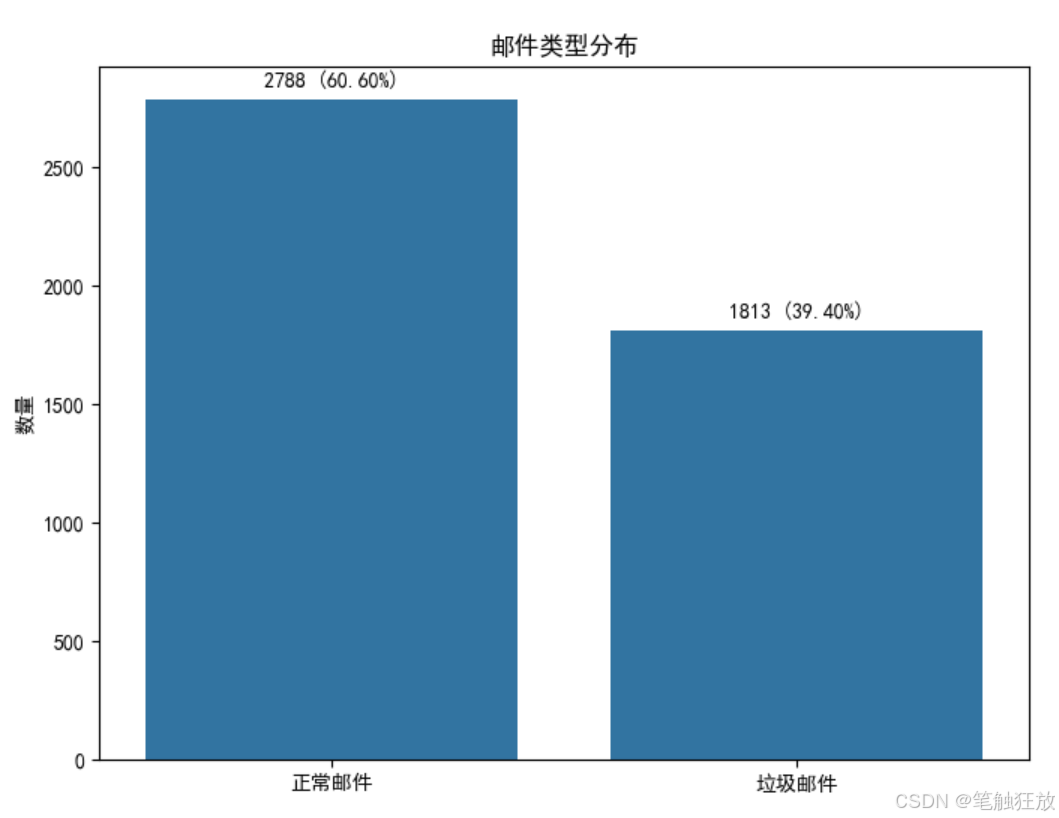
def visualize_data(self):
"""数据可视化"""
# 1. 垃圾邮件与正常邮件比例
plt.figure(figsize=(8, 6))
spam_counts = self.data['is_spam'].value_counts()
sns.barplot(x=['正常邮件', '垃圾邮件'], y=spam_counts.values)
plt.title('邮件类型分布')
plt.ylabel('数量')
for i, v in enumerate(spam_counts.values):
plt.text(i, v + 50, f'{v} ({v / len(self.data):.2%})', ha='center')
plt.show()
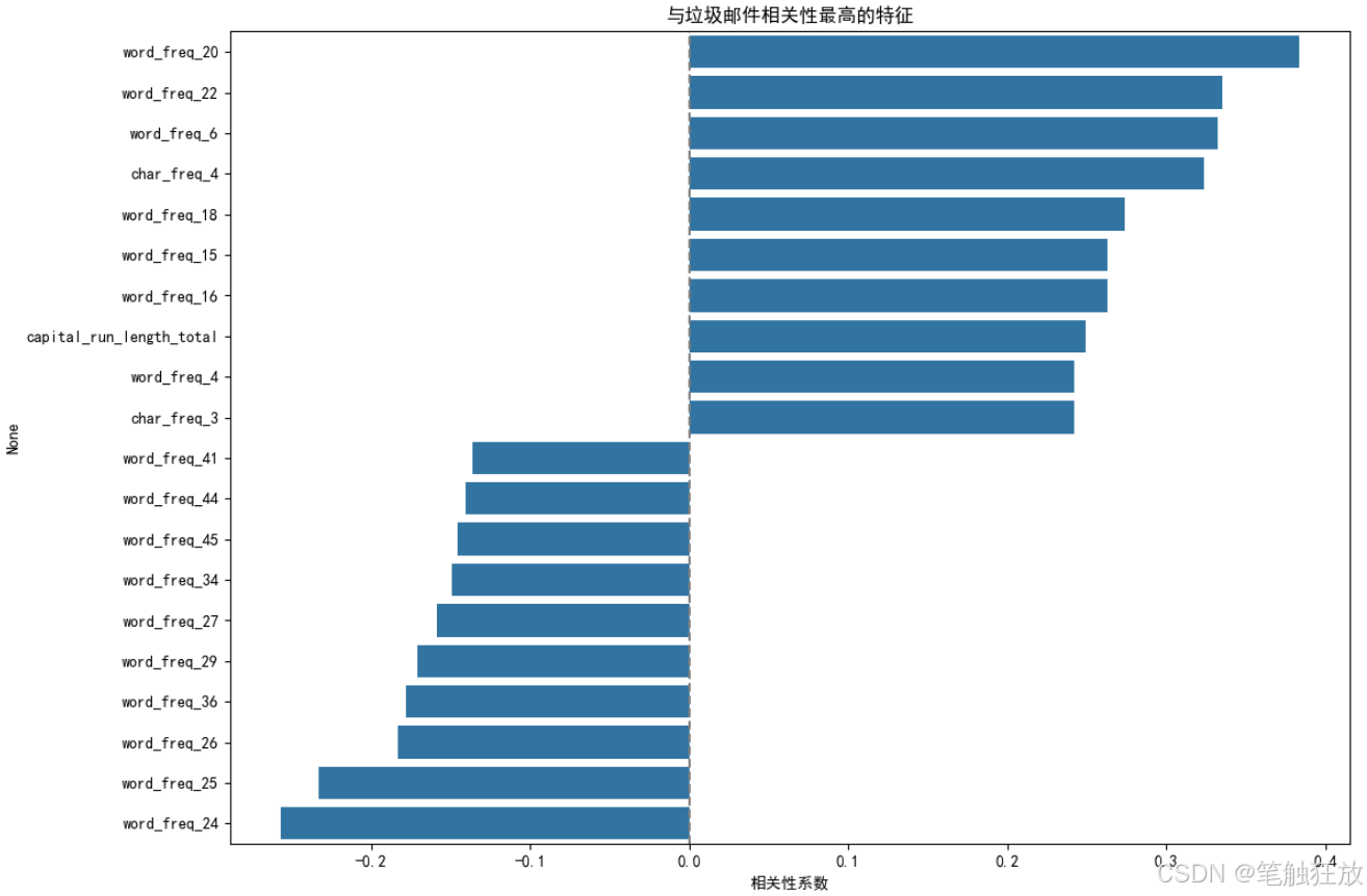
# 2. 最能区分垃圾邮件的特征
# 计算特征与垃圾邮件标签的相关性
correlations = self.data.corr()['is_spam'].sort_values(ascending=False)
# 取相关性最高和最低的各10个特征
top_features = pd.concat([correlations.head(11), correlations.tail(10)])
top_features = top_features.drop('is_spam') # 移除自身相关性
plt.figure(figsize=(12, 8))
sns.barplot(x=top_features.values, y=top_features.index)
plt.title('与垃圾邮件相关性最高的特征')
plt.xlabel('相关性系数')
plt.axvline(x=0, color='gray', linestyle='--')
plt.tight_layout()
plt.show()
def build_models(self):
"""构建多种分类模型"""
self.models = {
'朴素贝叶斯': MultinomialNB(),
'逻辑回归': LogisticRegression(max_iter=1000, random_state=42),
'支持向量机': SVC(probability=True, random_state=42),
'随机森林': RandomForestClassifier(random_state=42)
}
def train_models(self):
"""训练所有模型"""
print("\n=== 模型训练结果 ===")
for name, model in self.models.items():
# 训练模型
model.fit(self.X_train, self.y_train)
# 预测
y_pred = model.predict(self.X_test)
y_prob = model.predict_proba(self.X_test)[:, 1] # 预测为垃圾邮件的概率
# 保存结果
self.predictions[name] = y_pred
self.probabilities[name] = y_prob
# 计算准确率
accuracy = accuracy_score(self.y_test, y_pred)
print(f"{name} 准确率: {accuracy:.4f}")
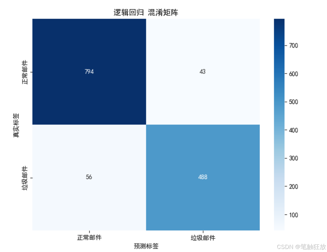
def evaluate_model(self, model_name):
"""详细评估指定模型"""
if model_name not in self.models:
print(f"模型 {model_name} 不存在,请先构建模型")
return
print(f"\n=== {model_name} 详细评估 ===")
# 1. 混淆矩阵
cm = confusion_matrix(self.y_test, self.predictions[model_name])
plt.figure(figsize=(8, 6))
sns.heatmap(cm, annot=True, fmt='d', cmap='Blues',
xticklabels=['正常邮件', '垃圾邮件'],
yticklabels=['正常邮件', '垃圾邮件'])
plt.xlabel('预测标签')
plt.ylabel('真实标签')
plt.title(f'{model_name} 混淆矩阵')
plt.show()
# 2. 分类报告
print("\n分类报告:")
print(classification_report(
self.y_test,
self.predictions[model_name],
target_names=['正常邮件', '垃圾邮件']
))
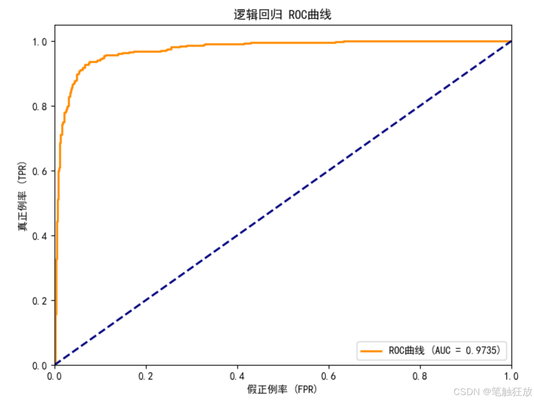
# 3. ROC曲线和AUC
fpr, tpr, _ = roc_curve(self.y_test, self.probabilities[model_name])
roc_auc = auc(fpr, tpr)
plt.figure(figsize=(8, 6))
plt.plot(fpr, tpr, color='darkorange', lw=2, label=f'ROC曲线 (AUC = {roc_auc:.4f})')
plt.plot([0, 1], [0, 1], color='navy', lw=2, linestyle='--')
plt.xlim([0.0, 1.0])
plt.ylim([0.0, 1.05])
plt.xlabel('假正例率 (FPR)')
plt.ylabel('真正例率 (TPR)')
plt.title(f'{model_name} ROC曲线')
plt.legend(loc="lower right")
plt.show()
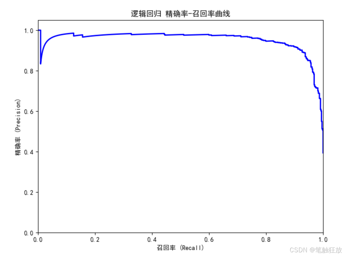
# 4. 精确率-召回率曲线
precision, recall, _ = precision_recall_curve(
self.y_test, self.probabilities[model_name]
)
plt.figure(figsize=(8, 6))
plt.plot(recall, precision, color='blue', lw=2)
plt.xlabel('召回率 (Recall)')
plt.ylabel('精确率 (Precision)')
plt.title(f'{model_name} 精确率-召回率曲线')
plt.xlim([0.0, 1.0])
plt.ylim([0.0, 1.05])
plt.show()
# 5. 交叉验证
cv_scores = cross_val_score(
self.models[model_name],
self.data.drop('is_spam', axis=1),
self.data['is_spam'],
cv=5
)
print(f"交叉验证准确率: {cv_scores.mean():.4f} (±{cv_scores.std():.4f})")
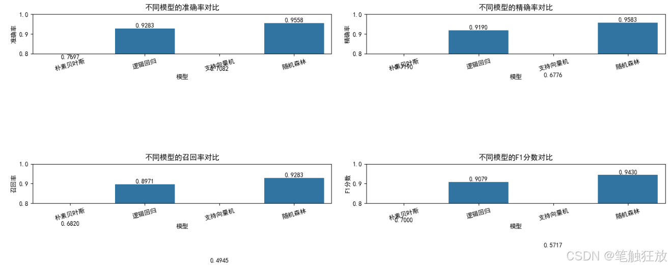
def compare_models(self):
"""比较所有模型的性能"""
# 收集各模型的评估指标
metrics = []
for name in self.models.keys():
report = classification_report(
self.y_test, self.predictions[name],
target_names=['正常邮件', '垃圾邮件'],
output_dict=True
)
metrics.append({
'模型': name,
'准确率': accuracy_score(self.y_test, self.predictions[name]),
'精确率': report['垃圾邮件']['precision'],
'召回率': report['垃圾邮件']['recall'],
'F1分数': report['垃圾邮件']['f1-score']
})
metrics_df = pd.DataFrame(metrics)
# 绘制各指标对比图
plt.figure(figsize=(15, 10))
for i, metric in enumerate(['准确率', '精确率', '召回率', 'F1分数']):
plt.subplot(2, 2, i + 1)
sns.barplot(x='模型', y=metric, data=metrics_df)
plt.title(f'不同模型的{metric}对比')
plt.ylim(0.8, 1.0) # 设置y轴范围以便更好地观察差异
for j, v in enumerate(metrics_df[metric]):
plt.text(j, v + 0.005, f'{v:.4f}', ha='center')
plt.xticks(rotation=15)
plt.tight_layout()
plt.show()
def optimize_model(self, model_name):
"""优化指定模型的超参数"""
if model_name not in self.models:
print(f"模型 {model_name} 不存在,请先构建模型")
return
print(f"\n=== 优化 {model_name} 超参数 ===")
# 定义参数网格
param_grids = {
'朴素贝叶斯': {'alpha': [0.1, 0.5, 1.0, 2.0, 5.0]},
'逻辑回归': {
'C': [0.01, 0.1, 1, 10, 100],
'penalty': ['l1', 'l2']
},
'支持向量机': {
'C': [0.1, 1, 10],
'kernel': ['linear', 'rbf'],
'gamma': ['scale', 'auto']
},
'随机森林': {
'n_estimators': [50, 100, 200],
'max_depth': [None, 10, 20],
'min_samples_split': [2, 5]
}
}
# 创建网格搜索对象
grid_search = GridSearchCV(
estimator=self.models[model_name],
param_grid=param_grids[model_name],
cv=5,
scoring='f1',
n_jobs=-1
)
# 执行网格搜索
grid_search.fit(self.X_train, self.y_train)
# 输出最佳参数
print(f"最佳参数: {grid_search.best_params_}")
# 评估优化后的模型
y_pred_opt = grid_search.predict(self.X_test)
print("\n优化后的分类报告:")
print(classification_report(
self.y_test, y_pred_opt,
target_names=['正常邮件', '垃圾邮件']
))
# 更新模型
self.models[model_name] = grid_search.best_estimator_
self.predictions[model_name] = y_pred_opt
self.probabilities[model_name] = grid_search.predict_proba(self.X_test)[:, 1]
return grid_search.best_estimator_
# 文本预处理函数(用于后续的原始邮件文本分类)
def preprocess_text(text):
"""预处理邮件文本"""
# 转换为小写
text = text.lower()
# 移除特殊字符和数字
text = re.sub(r'[^a-zA-Z\s]', '', text)
# 分词
words = text.split()
# 移除停用词并进行词形还原
lemmatizer = WordNetLemmatizer()
stop_words = set(stopwords.words('english'))
words = [lemmatizer.lemmatize(word) for word in words if word not in stop_words]
# 重新组合为字符串
return ' '.join(words)
# 基于原始文本的分类器(额外功能)
class TextBasedSpamClassifier:
def __init__(self):
# 加载原始邮件文本数据
self.load_text_data()
# 文本预处理
self.data['processed_text'] = self.data['text'].apply(preprocess_text)
# 划分训练集和测试集
X = self.data['processed_text']
y = self.data['is_spam']
self.X_train, self.X_test, self.y_train, self.y_test = train_test_split(
X, y, test_size=0.3, random_state=42, stratify=y
)
# 创建TF-IDF向量器和模型 pipeline
self.pipeline = Pipeline([
('tfidf', TfidfVectorizer(max_features=5000)),
('classifier', MultinomialNB())
])
def load_text_data(self):
"""加载原始邮件文本数据"""
print("\n正在加载原始邮件文本数据...")
# 使用简化的方式获取带文本的垃圾邮件数据
# 这里使用一个包含邮件文本和标签的示例数据集
# 实际应用中可以替换为自己的数据集
try:
# 尝试从公开URL加载数据
url = "https://raw.githubusercontent.com/justmarkham/pycon-2016-tutorial/master/data/sms.tsv"
self.data = pd.read_csv(url, sep='\t', header=None, names=['is_spam', 'text'])
self.data['is_spam'] = self.data['is_spam'].map({'ham': 0, 'spam': 1})
print(f"原始文本数据集加载完成,共 {self.data.shape[0]} 条短信")
except:
# 如果加载失败,使用模拟数据
print("无法加载远程数据,使用模拟数据")
texts = [
"Free money now! Click here",
"Hi, how are you doing?",
"Congratulations! You won a prize",
"Meeting tomorrow at 3pm",
"Get free access to our service",
"Can you send me the report?",
"Claim your discount today",
"Dinner tonight?",
"You have been selected for a free trial",
"Reminder: doctors appointment"
]
is_spam = [1, 0, 1, 0, 1, 0, 1, 0, 1, 0]
self.data = pd.DataFrame({'text': texts, 'is_spam': is_spam})
def train(self):
"""训练模型"""
print("训练基于文本的垃圾邮件分类器...")
self.pipeline.fit(self.X_train, self.y_train)
# 评估
y_pred = self.pipeline.predict(self.X_test)
print(f"基于文本的分类器准确率: {accuracy_score(self.y_test, y_pred):.4f}")
print("分类报告:")
print(classification_report(
self.y_test, y_pred,
target_names=['正常邮件', '垃圾邮件']
))
def predict(self, text):
"""预测单封邮件是否为垃圾邮件"""
processed = preprocess_text(text)
prediction = self.pipeline.predict([processed])[0]
probability = self.pipeline.predict_proba([processed])[0][1]
result = "垃圾邮件" if prediction == 1 else "正常邮件"
print(f"\n邮件内容: {text}")
print(f"预测结果: {result} (概率: {probability:.4f})")
return result
if __name__ == "__main__":
# 创建垃圾邮件分类器实例
classifier = SpamClassifier()
# 数据可视化
classifier.visualize_data()
# 构建并训练模型
classifier.build_models()
classifier.train_models()
# 比较所有模型
classifier.compare_models()
# 选择表现较好的模型进行详细评估(默认逻辑回归)
best_model = '逻辑回归'
classifier.evaluate_model(best_model)
# 优化最佳模型
classifier.optimize_model(best_model)
# 展示基于原始文本的分类器(额外功能)
text_classifier = TextBasedSpamClassifier()
text_classifier.train()
# 测试几个示例邮件
test_emails = [
"Congratulations! You've won a $1000 gift card. Click the link to claim now!",
"Hi John, are we still meeting for lunch tomorrow? Let me know.",
"Free entry in 2 a wkly comp to win FA Cup final tkts 21st May 2005. Text FA to 87121 to receive entry question(std txt rate)",
"Please find attached the report you requested. Let me know if you need any changes.",
"URGENT! Your account has been compromised. Click here to verify your information."
]
print("\n=== 测试邮件预测 ===")
for email in test_emails:
text_classifier.predict(email)这个垃圾邮件分类项目的主要功能和特点:
-
数据集选择:使用 UCI 的垃圾邮件数据集(Spambase),包含 4601 封邮件和 57 个特征,以及一个基于原始文本的 SMS 垃圾短信数据集
-
完整流程:实现了从数据加载、探索性分析、可视化、模型训练、评估到预测的完整流程
-
多种分类算法:包含朴素贝叶斯、逻辑回归、支持向量机和随机森林四种经典分类算法
-
丰富的可视化:提供邮件类型分布、特征相关性、混淆矩阵、ROC 曲线和精确率 - 召回率曲线等可视化图表
-
全面评估指标:使用准确率、精确率、召回率、F1 分数和 AUC 等指标评估模型性能
-
模型优化:实现了超参数网格搜索优化功能,提升模型性能
-
双重分类方式:
-
基于提取的特征(词频、字符频率等)进行分类
-
基于原始文本(使用 TF-IDF 向量化)进行分类
-
运行前需要安装以下依赖库:
pip install numpy pandas matplotlib seaborn scikit-learn nltk
程序运行后会:
-
展示数据集的基本信息和类别分布
-
生成多种可视化图表帮助理解数据特征
-
训练四种分类模型并比较它们的性能
-
对表现最佳的模型(默认逻辑回归)进行详细评估
-
优化最佳模型的超参数以获得更好的分类效果
-
额外提供基于原始文本的分类器,并对示例邮件进行预测
你可以通过修改test_emails列表中的内容来测试不同的邮件文本,观察模型的分类结果。这个项目对于理解文本分类、特征工程和机器学习模型在垃圾邮件检测中的应用非常有帮助。