#zhaoyunfei
###20251109
library(dplyr)
library(tidyr)
library(ggplot2)
library(sp)
library(reshape2)
# 设置参数
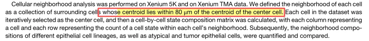
neighborhood_radius <- 80 # 邻域半径 80 μm
xenium_data <- readRDS("xenium_data.rds")
# 提取坐标和细胞类型信息
# 坐标在obj@meta.data的x,y列,细胞类型在celltype列
coordinates <- xenium_data@meta.data[, c("x", "y")]
celltypes <- xenium_data@meta.data$celltype
# 为每个细胞创建唯一标识符
cell_ids <- rownames(xenium_data@meta.data)
# 函数:计算两个点之间的欧几里得距离
calculate_distance <- function(point1, point2) {
sqrt((point1[1] - point2[1])^2 + (point1[2] - point2[2])^2)
}
# 函数:找到指定细胞周围80μm内的邻居细胞
find_neighbors <- function(center_cell_index, coordinates, radius) {
center_coord <- coordinates[center_cell_index, ]
distances <- apply(coordinates, 1, function(coord) {
calculate_distance(center_coord, coord)
})
neighbor_indices <- which(distances <= radius & distances > 0) # 排除自身
return(neighbor_indices)
}
# 创建细胞状态计数函数
count_cell_states <- function(neighbor_indices, celltypes) {
neighbor_celltypes <- celltypes[neighbor_indices]
celltype_table <- table(neighbor_celltypes)
return(celltype_table)
}
###构建细胞-by-细胞状态组成矩阵
# 初始化结果矩阵
all_celltypes <- unique(celltypes)
cell_state_matrix <- matrix(0,
nrow = length(all_celltypes),
ncol = length(cell_ids),
dimnames = list(all_celltypes, cell_ids))
#### 为每个细胞计算邻域组成
for (i in 1:length(cell_ids)) {
if (i %% 1000 == 0) cat("处理细胞:", i, "/", length(cell_ids), "\n")
##### 找到当前细胞的邻居
neighbor_indices <- find_neighbors(i, coordinates, neighborhood_radius)
if (length(neighbor_indices) > 0) {
# 计算邻域中的细胞状态组成
cellstate_counts <- count_cell_states(neighbor_indices, celltypes)
# 更新矩阵
for (celltype in names(cellstate_counts)) {
cell_state_matrix[celltype, i] <- cellstate_counts[celltype]
}
}
}
cat("细胞邻域组成矩阵构建完成!\n")
# 将矩阵转换为数据框便于分析
cell_state_df <- as.data.frame(t(cell_state_matrix))
cell_state_df$cell_id <- cell_ids
cell_state_df$center_celltype <- celltypes
cell_state_df$center_x <- coordinates$x
cell_state_df$center_y <- coordinates$y
# 分析特定上皮细胞谱系的邻域组成
# 假设我们关注的上皮细胞类型
epithelial_lineages <- c("Tumor_Epithelial", "Atypical_Epithelial", "Normal_Epithelial")
epithelial_lineages <- epithelial_lineages[epithelial_lineages %in% unique(celltypes)]
# 提取上皮细胞的邻域数据
epithelial_neighborhoods <- cell_state_df[cell_state_df$center_celltype %in% epithelial_lineages, ]
# 计算每种上皮细胞类型的平均邻域组成
epithelial_summary <- epithelial_neighborhoods %>%
group_by(center_celltype) %>%
summarise(across(all_celltypes, list(mean = mean, sd = sd), .names = "{.col}_{.fn}"))
# 可视化:比较不同上皮细胞类型的邻域组成
plot_data <- epithelial_neighborhoods %>%
select(center_celltype, all_of(all_celltypes)) %>%
pivot_longer(cols = all_of(all_celltypes),
names_to = "neighbor_celltype",
values_to = "count") %>%
group_by(center_celltype, neighbor_celltype) %>%
summarise(mean_count = mean(count),
se_count = sd(count) / sqrt(n()))
# 绘制热图显示邻域组成
heatmap_plot <- ggplot(plot_data, aes(x = center_celltype, y = neighbor_celltype, fill = mean_count)) +
geom_tile() +
scale_fill_gradient2(low = "blue", mid = "white", high = "red",
midpoint = mean(plot_data$mean_count)) +
labs(title = "细胞邻域组成热图",
x = "中心细胞类型",
y = "邻居细胞类型",
fill = "平均数量") +
theme_minimal() +
theme(axis.text.x = element_text(angle = 45, hjust = 1))
print(heatmap_plot)
# 绘制条形图比较主要细胞类型的分布
bar_plot <- ggplot(plot_data, aes(x = neighbor_celltype, y = mean_count, fill = center_celltype)) +
geom_bar(stat = "identity", position = "dodge") +
labs(title = "不同上皮细胞类型的邻域组成比较",
x = "邻居细胞类型",
y = "平均数量",
fill = "中心细胞类型") +
theme_minimal() +
theme(axis.text.x = element_text(angle = 45, hjust = 1))
print(bar_plot)
# 统计检验:比较不同上皮细胞类型的邻域组成差异
# 例如,比较肿瘤上皮细胞和非典型上皮细胞的邻域差异
if ("Tumor_Epithelial" %in% epithelial_lineages & "Atypical_Epithelial" %in% epithelial_lineages) {
# 对每种邻居细胞类型进行t检验
significant_differences <- list()
for (neighbor_type in all_celltypes) {
tumor_data <- epithelial_neighborhoods[epithelial_neighborhoods$center_celltype == "Tumor_Epithelial", neighbor_type]
atypical_data <- epithelial_neighborhoods[epithelial_neighborhoods$center_celltype == "Atypical_Epithelial", neighbor_type]
if (length(tumor_data) > 1 & length(atypical_data) > 1) {
t_test_result <- t.test(tumor_data, atypical_data)
if (t_test_result$p.value < 0.05) {
significant_differences[[neighbor_type]] <- list(
p_value = t_test_result$p.value,
mean_tumor = mean(tumor_data),
mean_atypical = mean(atypical_data)
)
}
}
}
cat("\n显著差异的邻居细胞类型:\n")
if (length(significant_differences) > 0) {
for (celltype in names(significant_differences)) {
cat(celltype, ": p =", significant_differences[[celltype]]$p_value,
"(Tumor:", round(significant_differences[[celltype]]$mean_tumor, 2),
"vs Atypical:", round(significant_differences[[celltype]]$mean_atypical, 2), ")\n")
}
} else {
cat("未发现显著差异\n")
}
}
# 保存结果
write.csv(cell_state_df, "cellular_neighborhood_composition.csv", row.names = FALSE)
write.csv(epithelial_summary, "epithelial_neighborhood_summary.csv", row.names = FALSE)
# 保存图表
ggsave("neighborhood_heatmap.png", heatmap_plot, width = 10, height = 8, dpi = 300)
ggsave("neighborhood_barchart.png", bar_plot, width = 12, height = 6, dpi = 300)
cat("分析完成! 结果已保存到当前工作目录。\n")