三维SDMTSP：遗传算法GA求解三维单仓库多旅行商问题，可以更改数据集和起点（MATLAB代码）

最近在研究三维单仓库多旅行商问题（3D-SDMTSP），这个问题在物流、无人机路径规划等领域都有广泛应用。简单来说，就是有多个旅行商从同一个仓库出发，去访问一系列的三维空间中的点，最终回到仓库。目标是最小化所有旅行商的总路径长度。听起来是不是有点像快递员送货的场景？

为了求解这个问题，我选择了遗传算法（GA），因为它在大规模搜索空间中的表现一直很稳定。当然，MATLAB作为我的主力工具，自然是首选。下面我就来分享一下我的思路和代码。

首先，我们需要定义问题的数据结构。假设我们有N个城市（或者说点），每个城市都有一个三维坐标。我们可以用一个N×3的矩阵来表示这些点的坐标。比如：

matlab 复制代码

cities = [
    0, 0, 0;
    1, 2, 3;
    4, 5, 6;
    7, 8, 9;
    % 更多城市...
];

接下来，我们需要定义遗传算法的参数，比如种群大小、迭代次数、交叉概率、变异概率等。这些参数可以根据具体问题调整，没有固定答案。

matlab 复制代码

popSize = 50; % 种群大小
maxGen = 100; % 最大迭代次数
crossProb = 0.8; % 交叉概率
mutProb = 0.1; % 变异概率

遗传算法的核心是种群进化。我们首先初始化一个随机的种群，每个个体代表一种旅行商的路径分配方案。然后通过选择、交叉、变异等操作，逐步优化种群。

matlab 复制代码

% 初始化种群
population = initPopulation(popSize, numCities, numSalesmen);

for gen = 1:maxGen
    % 计算适应度
    fitness = calculateFitness(population, cities);
    
    % 选择
    selectedPopulation = selection(population, fitness);
    
    % 交叉
    crossedPopulation = crossover(selectedPopulation, crossProb);
    
    % 变异
    mutatedPopulation = mutation(crossedPopulation, mutProb);
    
    % 更新种群
    population = mutatedPopulation;
end

这里的关键是适应度函数的计算。我们需要计算每个个体的总路径长度，路径越短，适应度越高。为了计算路径长度，我们可以使用欧几里得距离公式：

matlab 复制代码

function dist = calculateDistance(city1, city2)
    dist = sqrt(sum((city1 - city2).^2));
end

在交叉和变异操作中，我们需要确保每个旅行商的路径是有效的，不能有重复的城市。交叉可以采用部分映射交叉（PMX），变异可以采用交换变异。

matlab 复制代码

function newPopulation = crossover(population, crossProb)
    newPopulation = population;
    for i = 1:2:popSize
        if rand < crossProb
            % 选择交叉点
            crossPoint = randi([1, numCities]);
            % 执行交叉
            newPopulation(i, crossPoint:end) = population(i+1, crossPoint:end);
            newPopulation(i+1, crossPoint:end) = population(i, crossPoint:end);
        end
    end
end

function newPopulation = mutation(population, mutProb)
    newPopulation = population;
    for i = 1:popSize
        if rand < mutProb
            % 选择两个随机位置进行交换
            swapPositions = randperm(numCities, 2);
            newPopulation(i, swapPositions) = population(i, fliplr(swapPositions));
        end
    end
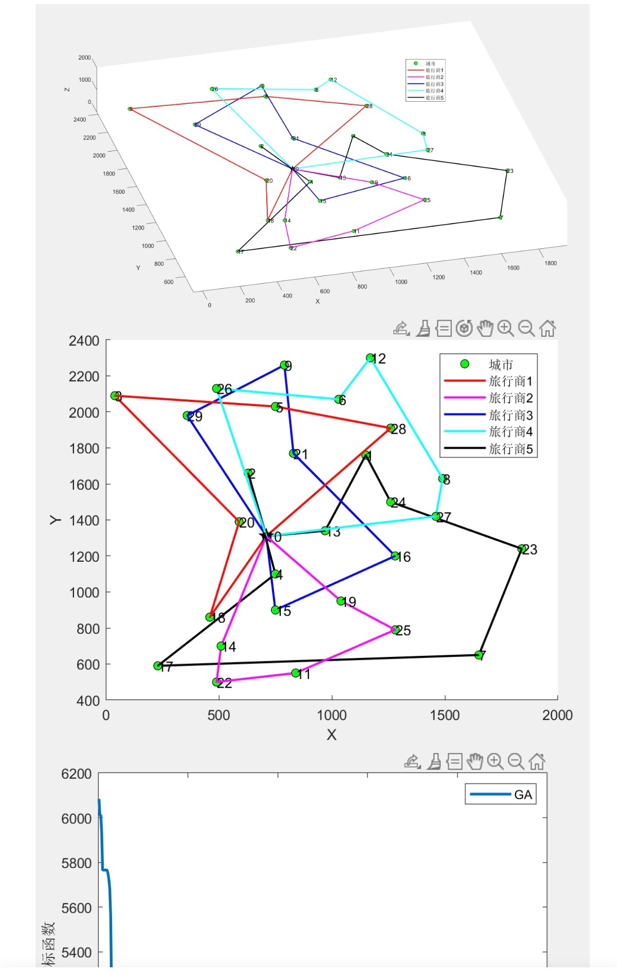
end

经过多次迭代后，种群中的最优个体就是我们想要的最优路径分配方案。我们可以通过可视化工具来展示最终的路径。

matlab 复制代码

% 获取最优个体
[~, bestIdx] = min(fitness);
bestSolution = population(bestIdx, :);

% 绘制路径
plot3(cities(:,1), cities(:,2), cities(:,3), 'o');
hold on;
for i = 1:numSalesmen
    path = bestSolution(i, :);
    plot3(cities(path, 1), cities(path, 2), cities(path, 3), '-');
end
hold off;

整个过程虽然看起来复杂，但通过遗传算法，我们能够有效地找到接近最优的解决方案。当然，遗传算法也有它的局限性，比如容易陷入局部最优，但通过调整参数和引入其他优化策略，我们可以进一步提升算法的性能。

如果你对这个问题的具体实现感兴趣，可以尝试修改数据集和起点，看看结果会有什么变化。毕竟，实践是检验真理的唯一标准嘛！