我来对这个决策逻辑图论系统进行深度详细解读。这个系统将粗糙集理论、决策逻辑和图论相结合,构建了一个强大的交互式分析工具。
一、系统架构概览
1.1 核心组件
1. DecisionTable    - 决策表(信息系统)
2. BipartiteGraph   - 二部图(表示逻辑公式)
3. DecisionLogicParser  - 决策逻辑解析器
4. RoughSetAnalyzer - 粗糙集分析器
5. Streamlit UI     - 交互式Web界面
1.2 技术栈
-
Streamlit:快速构建数据科学Web应用
-
NetworkX:图论计算(虽然这里用Plotly可视化)
-
Plotly:交互式可视化
-
Pandas/Numpy:数据处理
-
Python类型提示:增强代码可读性
二、核心类深度解析
2.1 DecisionTable(决策表)
作用:表示一个信息系统/决策表
关键数据结构:
class DecisionTable:
    def __init__(self, objects, attributes, values, decision_function):
        self.objects = objects          # 论域U = {x1, x2, ...}
        self.attributes = attributes    # 条件属性集合A = {a1, a2, ...}
        self.values = values           # 属性值域: {'颜色': ['红','蓝'], ...}
self.decision_function = decision_function # 映射: (对象,属性)→值数学模型:
-
决策表是四元组:
DT = (U, A, V, f) -
U: 论域(对象集合) -
A: 属性集合 -
V: 值域 -
f: U × A → V: 信息函数
关键方法:
-
get_value(obj, attr):获取对象在属性上的取值 -
get_equivalence_class(obj, attr):获取等价类-
等价类定义:
[x]_B = {y ∈ U | ∀a∈B, f(x,a)=f(y,a)} -
基于属性不可分辨关系
-
2.2 BipartiteGraph(二部图)
核心思想:用二部图表示决策逻辑公式的语义
图结构:
左部节点(对象节点):论域中的对象 {x1, x2, x3, ...}
右部节点(公式节点):逻辑公式 {φ, ψ, ...}
边:对象满足公式的关系关键操作:
2.2.1 翻转操作(逻辑非 ¬)
def flip(self) -> 'BipartiteGraph':
    # 语义:¬φ 表示所有不满足φ的对象满足¬φ
# 图论实现:原图中没有边的对象,在新图中有边数学原理:
-
公式φ的语义:
||φ|| = {x∈U | x ⊨ φ} -
非运算:
||¬φ|| = U - ||φ||
2.2.2 合取操作(逻辑与 ∧)
def conjunction(self, other) -> 'BipartiteGraph':
    # 语义:φ∧ψ 表示同时满足φ和ψ的对象
# 图论实现:取两个图中边的交集数学原理:
||φ∧ψ|| = ||φ|| ∩ ||ψ||
2.2.3 析取操作(逻辑或 ∨)
def disjunction(self, other) -> 'BipartiteGraph':
    # 语义:φ∨ψ 表示满足φ或ψ的对象
# 图论实现:取两个图中边的并集数学原理:
||φ∨ψ|| = ||φ|| ∪ ||ψ||
2.3 DecisionLogicParser(决策逻辑解析器)
作用:解析决策逻辑公式字符串,构建对应的二部图
语法定义:
原子公式: (属性,值)        如: (颜色,红)
复合公式: ¬φ, φ∧ψ, φ∨ψ 如: ¬(颜色,蓝)∧(形状,圆)解析过程:
-
原子公式解析 :
(颜色,红)→ 创建只包含该属性-值对的二部图 -
复合公式解析:递归下降解析
-
处理括号优先级
-
构建语法树
-
自底向上计算二部图
-
关键方法:
-
parse_formula(formula):主解析方法 -
_parse_atomic_formula():解析原子公式 -
_parse_composite_formula():解析复合公式
2.4 RoughSetAnalyzer(粗糙集分析器)
核心概念:粗糙集理论中的上下近似
数学定义:
-
下近似(Lower Approximation):
B*(X) = {x∈U | [x]_B ⊆ X}-
必然属于X的对象集合
-
等价类完全包含在X中
-
-
上近似(Upper Approximation):
B*(X) = {x∈U | [x]_B ∩ X ≠ ∅}-
可能属于X的对象集合
-
等价类与X有交集
-
实现算法:
def get_lower_approximation(formula_graph, attribute):
    # 1. 获取满足公式的对象集合X
    # 2. 获取属性B的等价类划分
    # 3. 找出所有等价类完全包含在X中的对象

def get_upper_approximation(formula_graph, attribute):
    # 1. 获取满足公式的对象集合X
    # 2. 获取属性B的等价类划分
# 3. 找出所有与X有交集的等价类近似精度:
α_B(X) = |B*(X)| / |B*(X)|-
衡量集合X的可定义程度
-
α=1:精确集(X可定义)
-
0<α<1:粗糙集(X不可定义)
三、系统工作流程
3.1 数据加载流程
1. 选择数据源(示例/CSV)
2. 构建DecisionTable对象
3. 预计算等价类缓存
4. 显示数据统计信息
3.2 公式分析流程
1. 用户输入公式:(颜色,红)∧(形状,圆)
2. 解析器构建二部图:
   - 解析(颜色,红) → 图G1
   - 解析(形状,圆) → 图G2
   - 计算G1 ∧ G2 → 结果图G
3. 粗糙集分析:
   - 选择属性B(如"颜色")
   - 计算等价类
   - 计算上下近似
4. 可视化展示
3.3 逻辑运算流程
输入:公式1=(颜色,红), 公式2=(形状,圆), 运算=∧
处理:
  1. 分别解析两个公式为二部图
  2. 调用conjunction方法合并
  3. 可视化合并结果
四、可视化系统详解
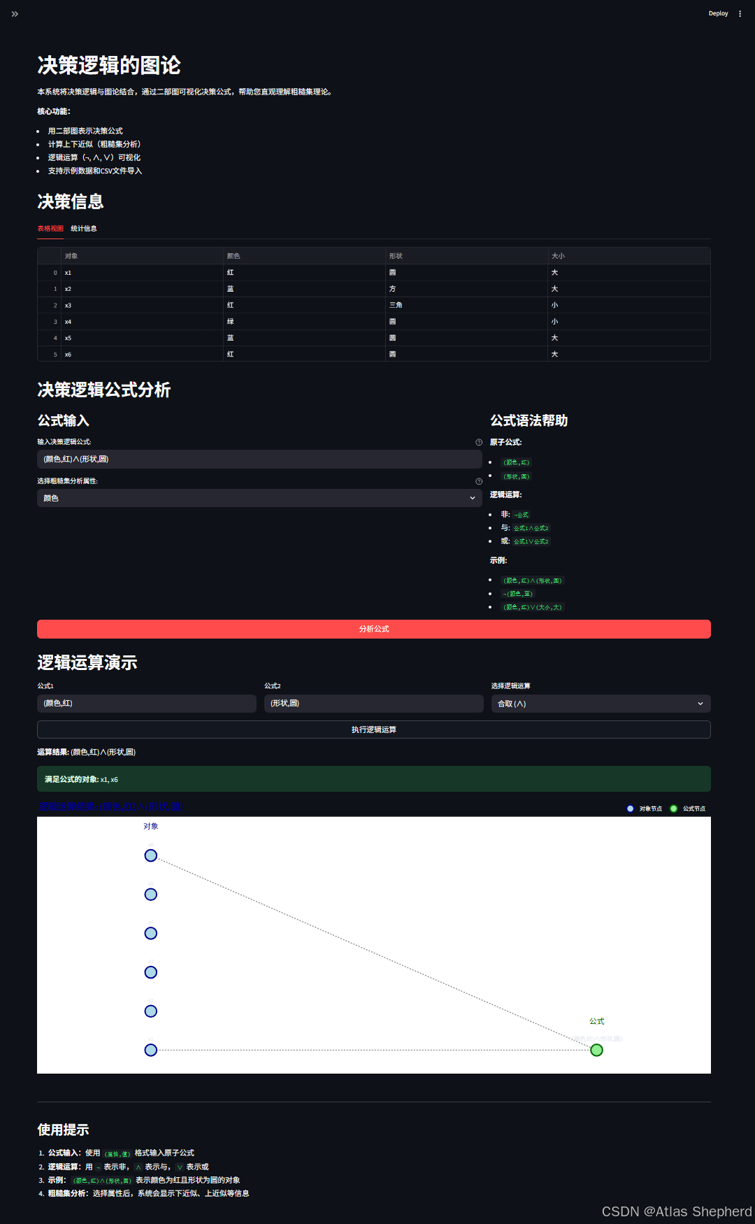
4.1 二部图可视化设计
布局策略:
-
左部节点:x=0,等间距垂直分布
-
右部节点:x=4,等间距垂直分布
-
边:虚线连接,增强可读性
视觉编码:
-
节点颜色:蓝色(对象)、绿色(公式)
-
边样式:灰色虚线
-
标签位置:节点上方
-
交互:悬停显示详细信息
4.2 多视图展示
-
表格视图:原始决策表
-
统计视图:数据概览
-
二部图视图:公式语义
-
分析视图:粗糙集结果
五、数学原理深度解析
5.1 决策逻辑的形式化定义
决策逻辑语言DL:
-
原子公式:
(a, v),其中a∈A, v∈V_a -
合式公式:
-
原子公式是合式公式
-
如果φ,ψ是合式公式,则¬φ, φ∧ψ, φ∨ψ是合式公式
-
语义解释:
-
x ⊨ (a, v)当且仅当f(x, a) = v -
x ⊨ ¬φ当且仅当 非(x ⊨ φ) -
x ⊨ φ∧ψ当且仅当x ⊨ φ且x ⊨ ψ -
x ⊨ φ∨ψ当且仅当x ⊨ φ或x ⊨ ψ
5.2 二部图与决策逻辑的对应关系
定理:每个决策逻辑公式φ都可以唯一对应一个二部图G(φ)
证明思路:
-
原子公式(a,v) → 二部图G,其中:
-
左节点:U
-
右节点:{(a,v)}
-
边:{(x, (a,v)) | f(x,a)=v}
-
-
复合公式:
-
¬φ → G(φ)的补图
-
φ∧ψ → G(φ)和G(ψ)的边交集
-
φ∨ψ → G(φ)和G(ψ)的边并集
-
5.3 粗糙集与二部图的联系
重要观察:
-
属性B的等价类划分对应一个划分二部图
-
公式φ的语义集||φ||对应一个二部图G(φ)
-
上下近似运算可以通过图操作实现
六、应用场景与扩展
6.1 实际应用
-
数据挖掘:发现决策规则
-
知识发现:从信息系统中提取知识
-
模式识别:识别对象类别
-
决策支持:辅助决策分析
6.2 系统扩展方向
# 1. 添加更多逻辑运算符
class ExtendedBipartiteGraph(BipartiteGraph):
    def implication(self, other):  # 蕴含 →
        return self.disjunction(other.flip())

    def equivalence(self, other):  # 等价 ↔
        return self.implication(other).conjunction(other.implication(self))

# 2. 支持更多粗糙集算子
def get_boundary_region(self, formula_graph, attribute):
    """边界域 = 上近似 - 下近似"""
    upper = self.get_upper_approximation(formula_graph, attribute)
    lower = self.get_lower_approximation(formula_graph, attribute)
    return upper - lower

# 3. 添加属性约简功能
def attribute_reduction(self, decision_attribute):
    """计算属性约简"""
    # 使用差别矩阵等方法
    pass
6.3 性能优化
-
缓存机制:已实现的等价类缓存
-
增量计算:避免重复计算
-
并行处理:多公式同时分析
-
图数据库:大规模图数据存储
七、完整代码
import streamlit as st
import networkx as nx
import plotly.graph_objects as go
import pandas as pd
import numpy as np
from typing import Dict, List, Set, Tuple, Any, Optional
import re
from io import StringIO
from dataclasses import dataclass
class DecisionTable:
"""决策表类,表示信息系统"""
def __init__(self, objects: List[str], attributes: List[str], values: Dict[str, List[str]],
decision_function: Dict[Tuple[str, str], str]):
self.objects = objects # 论域U
self.attributes = attributes # 属性集合A
self.values = values # 每个属性的可能取值 {属性: [值列表]}
self.decision_function = decision_function # 决策函数 f: (对象, 属性) -> 值
def get_value(self, obj: str, attr: str) -> str:
"""获取对象在某个属性上的值"""
return self.decision_function.get((obj, attr), "Unknown")
def get_equivalence_class(self, obj: str, attr: str) -> List[str]:
"""获取对象关于某个属性的等价类"""
target_value = self.get_value(obj, attr)
return [o for o in self.objects if self.get_value(o, attr) == target_value]
class BipartiteGraph:
"""二部图类"""
def __init__(self, left_nodes: Set[str], right_nodes: Set[str], edges: Set[Tuple[str, str]]):
self.left_nodes = left_nodes # 左部节点(通常是论域对象)
self.right_nodes = right_nodes # 右部节点(通常是公式或属性值)
self.edges = edges # 边集合
def flip(self) -> 'BipartiteGraph':
"""翻转操作(对应逻辑非)"""
# 处理空图情况:原公式为空(对所有对象都为假),翻转后为所有对象都满足
if not self.right_nodes:
return BipartiteGraph(
self.left_nodes,
{"True"}, # 表示恒真公式
{(obj, "True") for obj in self.left_nodes}
)
# 处理非空图
formula = next(iter(self.right_nodes)) # 安全获取第一个公式节点
new_right_nodes = {f"¬({formula})"}
# 翻转边:原图没有边的对象现在有边
new_edges = set()
for obj in self.left_nodes:
if not any(edge[0] == obj for edge in self.edges):
new_edges.add((obj, next(iter(new_right_nodes))))
return BipartiteGraph(self.left_nodes, new_right_nodes, new_edges)
def conjunction(self, other: 'BipartiteGraph') -> 'BipartiteGraph':
"""并操作(对应逻辑合取)"""
if self.left_nodes != other.left_nodes:
raise ValueError("两个二部图的左部节点必须相同")
# 处理空图情况
if not self.right_nodes:
return other # 空公式 ∧ X = X
if not other.right_nodes:
return self # X ∧ 空公式 = X
formula1 = next(iter(self.right_nodes))
formula2 = next(iter(other.right_nodes))
new_right_nodes = {f"({formula1}∧{formula2})"}
# 只有两个原图中都有边的节点在新图中有边
new_edges = set()
for obj in self.left_nodes:
if (obj, formula1) in self.edges and (obj, formula2) in other.edges:
new_edges.add((obj, next(iter(new_right_nodes))))
return BipartiteGraph(self.left_nodes, new_right_nodes, new_edges)
def disjunction(self, other: 'BipartiteGraph') -> 'BipartiteGraph':
"""或操作(对应逻辑析取)"""
if self.left_nodes != other.left_nodes:
raise ValueError("两个二部图的左部节点必须相同")
# 处理空图情况
if not self.right_nodes:
return other # 空公式 ∨ X = X
if not other.right_nodes:
return self # X ∨ 空公式 = X
formula1 = next(iter(self.right_nodes))
formula2 = next(iter(other.right_nodes))
new_right_nodes = {f"({formula1}∨{formula2})"}
# 只要有一个原图中有边的节点在新图中就有边
new_edges = set()
for obj in self.left_nodes:
if (obj, formula1) in self.edges or (obj, formula2) in other.edges:
new_edges.add((obj, next(iter(new_right_nodes))))
return BipartiteGraph(self.left_nodes, new_right_nodes, new_edges)
def visualize(self, title: str = "二部图") -> go.Figure:
"""使用Plotly可视化二部图,增强可读性"""
# 创建图形对象
fig = go.Figure()
# 准备节点位置
left_nodes_sorted = sorted(self.left_nodes)
right_nodes_sorted = sorted(self.right_nodes)
# 处理空图
if not left_nodes_sorted or not right_nodes_sorted:
fig.update_layout(
title=dict(text=f"{title} (空图)", font=dict(size=20, color='darkblue')),
xaxis=dict(showgrid=False, zeroline=False, showticklabels=False),
yaxis=dict(showgrid=False, zeroline=False, showticklabels=False),
plot_bgcolor='white',
height=400
)
return fig
# 左部节点位置(左侧)
left_positions = {}
for i, node in enumerate(left_nodes_sorted):
left_positions[node] = (0, i * 2) # x=0, y递增
# 右部节点位置(右侧)
right_positions = {}
for i, node in enumerate(right_nodes_sorted):
right_positions[node] = (4, i * 2) # x=4, y递增
# 所有节点位置
node_positions = {**left_positions, **right_positions}
# 添加边
edge_x = []
edge_y = []
for edge in self.edges:
if edge[0] in node_positions and edge[1] in node_positions:
x0, y0 = node_positions[edge[0]]
x1, y1 = node_positions[edge[1]]
# 添加边(用直线)
edge_x.extend([x0, x1, None])
edge_y.extend([y0, y1, None])
# 添加边的轨迹
if edge_x:
fig.add_trace(go.Scatter(
x=edge_x,
y=edge_y,
mode='lines',
line=dict(width=2, color='#888', dash='dot'),
hoverinfo='none',
showlegend=False,
name='边'
))
# 添加左部节点(对象节点)
left_node_x = [left_positions[node][0] for node in left_nodes_sorted]
left_node_y = [left_positions[node][1] for node in left_nodes_sorted]
fig.add_trace(go.Scatter(
x=left_node_x,
y=left_node_y,
mode='markers+text',
text=left_nodes_sorted,
textposition="top center",
marker=dict(
size=25,
color='lightblue',
line=dict(width=3, color='darkblue')
),
name='对象节点',
hoverinfo='text',
hovertext=[f"对象: {node}" for node in left_nodes_sorted]
))
# 添加右部节点(公式节点)
right_node_x = [right_positions[node][0] for node in right_nodes_sorted]
right_node_y = [right_positions[node][1] for node in right_nodes_sorted]
fig.add_trace(go.Scatter(
x=right_node_x,
y=right_node_y,
mode='markers+text',
text=right_nodes_sorted,
textposition="top center",
marker=dict(
size=25,
color='lightgreen',
line=dict(width=3, color='darkgreen')
),
name='公式节点',
hoverinfo='text',
hovertext=[f"公式: {node}" for node in right_nodes_sorted]
))
# 更新布局
fig.update_layout(
title=dict(
text=title,
font=dict(size=20, color='darkblue')
),
showlegend=True,
hovermode='closest',
margin=dict(b=20, l=5, r=5, t=40),
xaxis=dict(showgrid=False, zeroline=False, showticklabels=False, range=[-1, 5]),
yaxis=dict(showgrid=False, zeroline=False, showticklabels=False),
plot_bgcolor='white',
height=600,
annotations=[
dict(
text="对象",
x=0,
y=max(left_node_y) + 1.5 if left_node_y else 1,
showarrow=False,
font=dict(size=16, color='darkblue')
),
dict(
text="公式",
x=4,
y=max(right_node_y) + 1.5 if right_node_y else 1,
showarrow=False,
font=dict(size=16, color='darkgreen')
)
],
# 添加图例说明
legend=dict(
orientation="h",
yanchor="bottom",
y=1.02,
xanchor="right",
x=1
)
)
return fig
def get_satisfying_objects(self) -> Set[str]:
"""获取满足公式的对象集合"""
return {edge[0] for edge in self.edges}
class DecisionLogicParser:
"""决策逻辑公式解析器"""
def __init__(self, decision_table: DecisionTable):
self.decision_table = decision_table
self.atomic_graphs = self._create_atomic_graphs()
def _create_atomic_graphs(self) -> Dict[str, BipartiteGraph]:
"""创建基本原子公式的二部图"""
graphs = {}
for attr in self.decision_table.attributes:
left_nodes = set(self.decision_table.objects)
right_nodes = set()
edges = set()
for value in self.decision_table.values.get(attr, []):
formula = f"({attr},{value})"
right_nodes.add(formula)
# 添加边:对象与它对应的属性值相连
for obj in self.decision_table.objects:
if self.decision_table.get_value(obj, attr) == value:
edges.add((obj, formula))
graphs[attr] = BipartiteGraph(left_nodes, right_nodes, edges)
return graphs
def parse_formula(self, formula: str) -> BipartiteGraph:
"""解析决策逻辑公式并返回对应的二部图"""
formula = formula.replace(' ', '') # 移除空格
# 处理空公式
if not formula:
return BipartiteGraph(set(), set(), set())
# 处理原子公式
atomic_graph = self._parse_atomic_formula(formula)
if atomic_graph is not None:
return atomic_graph
# 处理复合公式
return self._parse_composite_formula(formula)
def _parse_atomic_formula(self, formula: str) -> Optional[BipartiteGraph]:
"""解析原子公式"""
# 原子公式:格式为 (属性,值)
atomic_pattern = r'\((\w+),(\w+)\)'
atomic_match = re.match(f'^{atomic_pattern}$', formula)
if atomic_match:
attr, value = atomic_match.group(1), atomic_match.group(2)
if attr in self.atomic_graphs:
# 从属性图中提取特定的原子公式图
base_graph = self.atomic_graphs[attr]
# 找到对应的公式节点
target_node = None
for node in base_graph.right_nodes:
if f"({attr},{value})" == node:
target_node = node
break
if target_node:
# 创建只包含该特定公式的边
edges = {(left, target_node) for left in base_graph.left_nodes
if (left, target_node) in base_graph.edges}
return BipartiteGraph(base_graph.left_nodes, {target_node}, edges)
return None
def _parse_composite_formula(self, formula: str) -> BipartiteGraph:
"""解析复合公式"""
# 处理逻辑非
if formula.startswith('¬'):
sub_formula = formula[1:]
# 如果子公式被括号包围,去掉括号
if sub_formula.startswith('(') and sub_formula.endswith(')'):
sub_formula = sub_formula[1:-1]
sub_graph = self.parse_formula(sub_formula)
return sub_graph.flip()
# 处理合取和析取
# 先找到最外层的主运算符(不在括号内)
depth = 0
for i, char in enumerate(formula):
if char == '(':
depth += 1
elif char == ')':
depth -= 1
elif depth == 0:
if char == '∧':
left_formula = formula[:i]
right_formula = formula[i + 1:]
left_graph = self.parse_formula(left_formula)
right_graph = self.parse_formula(right_formula)
return left_graph.conjunction(right_graph)
elif char == '∨':
left_formula = formula[:i]
right_formula = formula[i + 1:]
left_graph = self.parse_formula(left_formula)
right_graph = self.parse_formula(right_formula)
return left_graph.disjunction(right_graph)
# 如果公式被括号包围,去掉括号并重新解析
if formula.startswith('(') and formula.endswith(')'):
return self.parse_formula(formula[1:-1])
raise ValueError(f"无法解析公式: {formula}. 请检查语法,示例: (颜色,红)∧(形状,圆)")
class RoughSetAnalyzer:
"""粗糙集分析器"""
def __init__(self, decision_table: DecisionTable):
self.decision_table = decision_table
# 预计算等价类以提高效率
self.equivalence_classes_cache = {}
def _get_equivalence_classes(self, attribute: str) -> Dict[str, Set[str]]:
"""获取属性对应的所有等价类"""
if attribute not in self.equivalence_classes_cache:
classes = {}
for obj in self.decision_table.objects:
equiv_class = set(self.decision_table.get_equivalence_class(obj, attribute))
# 使用排序后的元组作为键,确保相同的等价类被合并
key = tuple(sorted(equiv_class))
if key not in classes:
classes[key] = equiv_class
self.equivalence_classes_cache[attribute] = classes
return self.equivalence_classes_cache[attribute]
def get_lower_approximation(self, formula_graph: BipartiteGraph, attribute: str) -> Set[str]:
"""计算下近似(必然为真的对象)"""
lower_approx = set()
satisfying_objects = formula_graph.get_satisfying_objects()
# 获取所有等价类
equivalence_classes = self._get_equivalence_classes(attribute)
for equiv_class in equivalence_classes.values():
# 如果等价类中的所有对象都满足公式
if equiv_class.issubset(satisfying_objects):
lower_approx.update(equiv_class)
return lower_approx
def get_upper_approximation(self, formula_graph: BipartiteGraph, attribute: str) -> Set[str]:
"""计算上近似(可能为真的对象)"""
upper_approx = set()
satisfying_objects = formula_graph.get_satisfying_objects()
# 获取所有等价类
equivalence_classes = self._get_equivalence_classes(attribute)
for equiv_class in equivalence_classes.values():
# 如果等价类中至少有一个对象满足公式
if not equiv_class.isdisjoint(satisfying_objects):
upper_approx.update(equiv_class)
return upper_approx
def create_sample_decision_table() -> DecisionTable:
"""创建示例决策表"""
objects = ['x1', 'x2', 'x3', 'x4', 'x5', 'x6']
attributes = ['颜色', '形状', '大小']
values = {
'颜色': ['红', '蓝', '绿'],
'形状': ['圆', '方', '三角'],
'大小': ['大', '小']
}
# 决策函数数据
data = {
('x1', '颜色'): '红', ('x1', '形状'): '圆', ('x1', '大小'): '大',
('x2', '颜色'): '蓝', ('x2', '形状'): '方', ('x2', '大小'): '大',
('x3', '颜色'): '红', ('x3', '形状'): '三角', ('x3', '大小'): '小',
('x4', '颜色'): '绿', ('x4', '形状'): '圆', ('x4', '大小'): '小',
('x5', '颜色'): '蓝', ('x5', '形状'): '圆', ('x5', '大小'): '大',
('x6', '颜色'): '红', ('x6', '形状'): '圆', ('x6', '大小'): '大'
}
return DecisionTable(objects, attributes, values, data)
def load_decision_table_from_csv(uploaded_file) -> Optional[DecisionTable]:
"""从CSV文件加载决策表"""
try:
df = pd.read_csv(uploaded_file)
if df.empty:
return None
objects = df.iloc[:, 0].tolist() # 第一列作为对象
attributes = df.columns[1:].tolist() # 其余列作为属性
values = {}
decision_function = {}
for attr in attributes:
unique_values = df[attr].dropna().unique().tolist()
values[attr] = [str(v) for v in unique_values]
for idx, obj in enumerate(objects):
decision_function[(obj, attr)] = str(df.iloc[idx][df.columns.get_loc(attr)])
return DecisionTable(objects, attributes, values, decision_function)
except Exception as e:
st.error(f"加载CSV文件时出错: {e}")
return None
def main():
st.set_page_config(page_title="决策逻辑图论", page_icon="📊", layout="wide")
st.title("决策逻辑的图论")
st.markdown("""
本系统将决策逻辑与图论结合,通过二部图可视化决策公式,帮助您直观理解粗糙集理论。
**核心功能:**
- 用二部图表示决策公式
- 计算上下近似(粗糙集分析)
- 逻辑运算(¬, ∧, ∨)可视化
- 支持示例数据和CSV文件导入
""")
# 侧边栏配置
st.sidebar.header("系统配置")
# 数据加载选项
data_option = st.sidebar.radio("选择数据源:",
["使用示例数据", "上传CSV文件"])
decision_table = None
if data_option == "使用示例数据":
decision_table = create_sample_decision_table()
st.sidebar.success("已加载示例数据")
# 显示示例数据详情
with st.sidebar.expander("示例数据详情"):
st.write("**对象:** " + ", ".join(decision_table.objects))
st.write("**属性:** " + ", ".join(decision_table.attributes))
for attr in decision_table.attributes:
st.write(f"**{attr}的取值:** " + ", ".join(decision_table.values.get(attr, [])))
else:
uploaded_file = st.sidebar.file_uploader("上传CSV文件", type=['csv'])
if uploaded_file is not None:
decision_table = load_decision_table_from_csv(uploaded_file)
if decision_table:
st.sidebar.success(
f"CSV文件加载成功: {len(decision_table.objects)}个对象, {len(decision_table.attributes)}个属性")
if decision_table is None:
st.info("请先加载数据以开始分析")
return
# 显示决策表
st.header("决策信息")
# 创建交互式数据展示
tab1, tab2 = st.tabs(["表格视图", "统计信息"])
with tab1:
# 创建表格显示
table_data = []
for obj in decision_table.objects:
row = [obj]
for attr in decision_table.attributes:
row.append(decision_table.get_value(obj, attr))
table_data.append(row)
df_display = pd.DataFrame(table_data,
columns=['对象'] + decision_table.attributes)
st.dataframe(df_display, use_container_width=True)
with tab2:
col1, col2, col3 = st.columns(3)
with col1:
st.metric("论域对象数", len(decision_table.objects))
with col2:
st.metric("属性数", len(decision_table.attributes))
with col3:
total_values = sum(len(vals) for vals in decision_table.values.values())
st.metric("属性值总数", total_values)
# 显示属性详情
st.subheader("属性详情")
for attr in decision_table.attributes:
with st.expander(f"属性: {attr}"):
values = decision_table.values.get(attr, [])
st.write(f"**可能取值:** {', '.join(values)}")
# 显示每个值的对象分布
for value in values:
count = sum(1 for obj in decision_table.objects
if decision_table.get_value(obj, attr) == value)
st.write(f"- {value}: {count}个对象")
# 公式解析和可视化
st.header("决策逻辑公式分析")
col1, col2 = st.columns([2, 1])
with col1:
st.subheader("公式输入")
formula_input = st.text_input(
"输入决策逻辑公式:",
value="(颜色,红)∧(形状,圆)",
help="支持格式: (属性,值), 以及¬, ∧, ∨操作。示例: ¬(颜色,蓝)∧(形状,圆)"
)
selected_attribute = st.selectbox(
"选择粗糙集分析属性:",
decision_table.attributes,
help="用于计算上下近似的属性"
)
with col2:
st.subheader("公式语法帮助")
st.markdown("""
**原子公式:**
- `(颜色,红)`
- `(形状,圆)`
**逻辑运算:**
- 非: `¬公式`
- 与: `公式1∧公式2`
- 或: `公式1∨公式2`
**示例:**
- `(颜色,红)∧(形状,圆)`
- `¬(颜色,蓝)`
- `(颜色,红)∨(大小,大)`
""")
if st.button("分析公式", type="primary", use_container_width=True):
try:
# 初始化解析器和分析器
parser = DecisionLogicParser(decision_table)
analyzer = RoughSetAnalyzer(decision_table)
# 解析公式
with st.spinner("解析公式中..."):
formula_graph = parser.parse_formula(formula_input)
# 计算粗糙集近似
with st.spinner("计算粗糙集近似中..."):
lower_approx = analyzer.get_lower_approximation(formula_graph, selected_attribute)
upper_approx = analyzer.get_upper_approximation(formula_graph, selected_attribute)
# 显示结果
st.subheader("分析结果")
result_col1, result_col2, result_col3 = st.columns(3)
with result_col1:
satisfying_count = len(formula_graph.get_satisfying_objects())
st.metric("满足公式的对象数", satisfying_count)
with result_col2:
st.metric("下近似(必然真)", len(lower_approx))
with result_col3:
st.metric("上近似(可能真)", len(upper_approx))
# 显示详细信息
st.subheader("详细结果")
col1, col2 = st.columns(2)
with col1:
st.write("**满足公式的对象:**")
satisfying_objects = formula_graph.get_satisfying_objects()
if satisfying_objects:
st.success(", ".join(sorted(satisfying_objects)))
else:
st.warning("无")
st.write("**下近似对象(必然真):**")
if lower_approx:
st.success(", ".join(sorted(lower_approx)))
else:
st.info("无")
st.write("**上近似对象(可能真):**")
if upper_approx:
st.info(", ".join(sorted(upper_approx)))
else:
st.warning("无")
with col2:
st.write("**边界域对象(不确定):**")
boundary = upper_approx - lower_approx
if boundary:
st.warning(", ".join(sorted(boundary)))
else:
st.success("无(精确集)")
st.write("**负域对象(必然假):**")
negative = set(decision_table.objects) - upper_approx
if negative:
st.error(", ".join(sorted(negative)))
else:
st.success("无")
# 计算近似精度
if upper_approx:
precision = len(lower_approx) / len(upper_approx)
st.metric("近似精度", f"{precision:.2%}")
# 使用Plotly可视化
st.subheader("二部图可视化")
fig = formula_graph.visualize(f"公式 '{formula_input}' 的二部图语义")
st.plotly_chart(fig, use_container_width=True)
# 显示图结构信息
with st.expander("图结构详情"):
st.write(f"**左部节点数(对象):** {len(formula_graph.left_nodes)}")
st.write(f"**右部节点数(公式):** {len(formula_graph.right_nodes)}")
st.write(f"**边数:** {len(formula_graph.edges)}")
if formula_graph.edges:
st.write("**边列表:**")
for edge in sorted(formula_graph.edges):
st.write(f" {edge[0]} ↔ {edge[1]}")
else:
st.write("**边列表:** 无")
# 显示等价类信息
st.subheader("等价类分析")
equivalence_classes = analyzer._get_equivalence_classes(selected_attribute)
for i, (key, equiv_class) in enumerate(list(equivalence_classes.items())[:3]):
st.write(f"**等价类 {i + 1}** ({len(equiv_class)}个对象): {', '.join(sorted(equiv_class))}")
# 检查该等价类与公式的关系
if equiv_class.issubset(satisfying_objects):
st.success("✓ 整个等价类都满足公式(属于下近似)")
elif not equiv_class.isdisjoint(satisfying_objects):
st.info("✓ 等价类中部分对象满足公式(属于上近似)")
else:
st.error("✗ 等价类中没有对象满足公式(属于负域)")
if len(equivalence_classes) > 3:
st.info(f"还有 {len(equivalence_classes) - 3} 个等价类未显示...")
except Exception as e:
st.error(f"公式分析错误: {str(e)}")
st.info("请检查公式语法是否正确。确保使用正确的格式,如: `(属性,值)`,并注意括号匹配。")
# 逻辑运算演示
st.header("逻辑运算演示")
col1, col2, col3 = st.columns(3)
with col1:
formula1 = st.text_input("公式1", value="(颜色,红)", key="formula1")
with col2:
formula2 = st.text_input("公式2", value="(形状,圆)", key="formula2")
with col3:
operation = st.selectbox(
"选择逻辑运算",
["合取 (∧)", "析取 (∨)", "非 (¬)"],
key="operation"
)
if st.button("执行逻辑运算", key="execute_op", use_container_width=True):
try:
parser = DecisionLogicParser(decision_table)
if operation == "非 (¬)":
formula = f"¬{formula1}"
with st.spinner(f"计算 {formula} 中..."):
result_graph = parser.parse_formula(formula)
st.write(f"**运算结果:** {formula}")
else:
if operation == "合取 (∧)":
formula = f"{formula1}∧{formula2}"
with st.spinner(f"计算 {formula} 中..."):
graph1 = parser.parse_formula(formula1)
graph2 = parser.parse_formula(formula2)
result_graph = graph1.conjunction(graph2)
else: # 析取
formula = f"{formula1}∨{formula2}"
with st.spinner(f"计算 {formula} 中..."):
graph1 = parser.parse_formula(formula1)
graph2 = parser.parse_formula(formula2)
result_graph = graph1.disjunction(graph2)
st.write(f"**运算结果:** {formula}")
# 显示结果
satisfying_objects = result_graph.get_satisfying_objects()
if satisfying_objects:
st.success(f"**满足公式的对象:** {', '.join(sorted(satisfying_objects))}")
else:
st.warning("没有对象满足该公式")
# 可视化结果
fig = result_graph.visualize(f"逻辑运算结果: {formula}")
st.plotly_chart(fig, use_container_width=True)
except Exception as e:
st.error(f"逻辑运算错误: {str(e)}")
st.info("请确保输入的公式格式正确,例如: (颜色,红) 或 ¬(形状,方)")
# 系统信息
st.sidebar.markdown("---")
st.sidebar.header("系统信息")
st.sidebar.info("""
**决策逻辑图论系统**
- 基于粗糙集理论的决策逻辑可视化
- 二部图表示决策公式
- 支持逻辑运算和粗糙集分析
- 2025年12月最新版
""")
# 添加使用提示
st.markdown("""
---
### 使用提示
1. **公式输入**:使用 `(属性,值)` 格式输入原子公式
2. **逻辑运算**:用 `¬` 表示非,`∧` 表示与,`∨` 表示或
3. **示例**:`(颜色,红)∧(形状,圆)` 表示颜色为红且形状为圆的对象
4. **粗糙集分析**:选择属性后,系统会显示下近似、上近似等信息
""")
if __name__ == "__main__":
main()