【深度学习实战】突破灾难性遗忘！基于经验回放+EWC的核电站故障诊断增量学习系统完整实现

突破灾难性遗忘！基于经验回放+EWC的核电站故障诊断增量学习系统完整实现资源-CSDN下载

一、引言：当AI遇到"遗忘症"------灾难性遗忘的挑战

在深度学习领域，有一个令人头疼的问题：灾难性遗忘（Catastrophic Forgetting）。想象一下，你训练了一个能够识别10种核电站故障的智能诊断系统，准确率高达95%。但是，当系统需要学习第11种新故障时，悲剧发生了------它突然忘记了之前学过的所有故障类型，准确率暴跌到30%以下。这就是灾难性遗忘的残酷现实。

在核电站这样的关键基础设施中，故障诊断系统必须能够：

• 持续学习：随着设备老化、运行条件变化，不断出现新的故障模式

• 保持记忆：不能忘记已经学过的历史故障类型

• 实时部署：不能每次都重新训练整个模型（计算成本和时间成本都太高）

传统的机器学习方法在面对这个问题时显得力不从心。每次新增故障类型，都需要：

• 重新收集所有历史数据

• 重新训练整个模型（可能需要数天甚至数周）

• 重新部署系统（停机时间成本巨大）

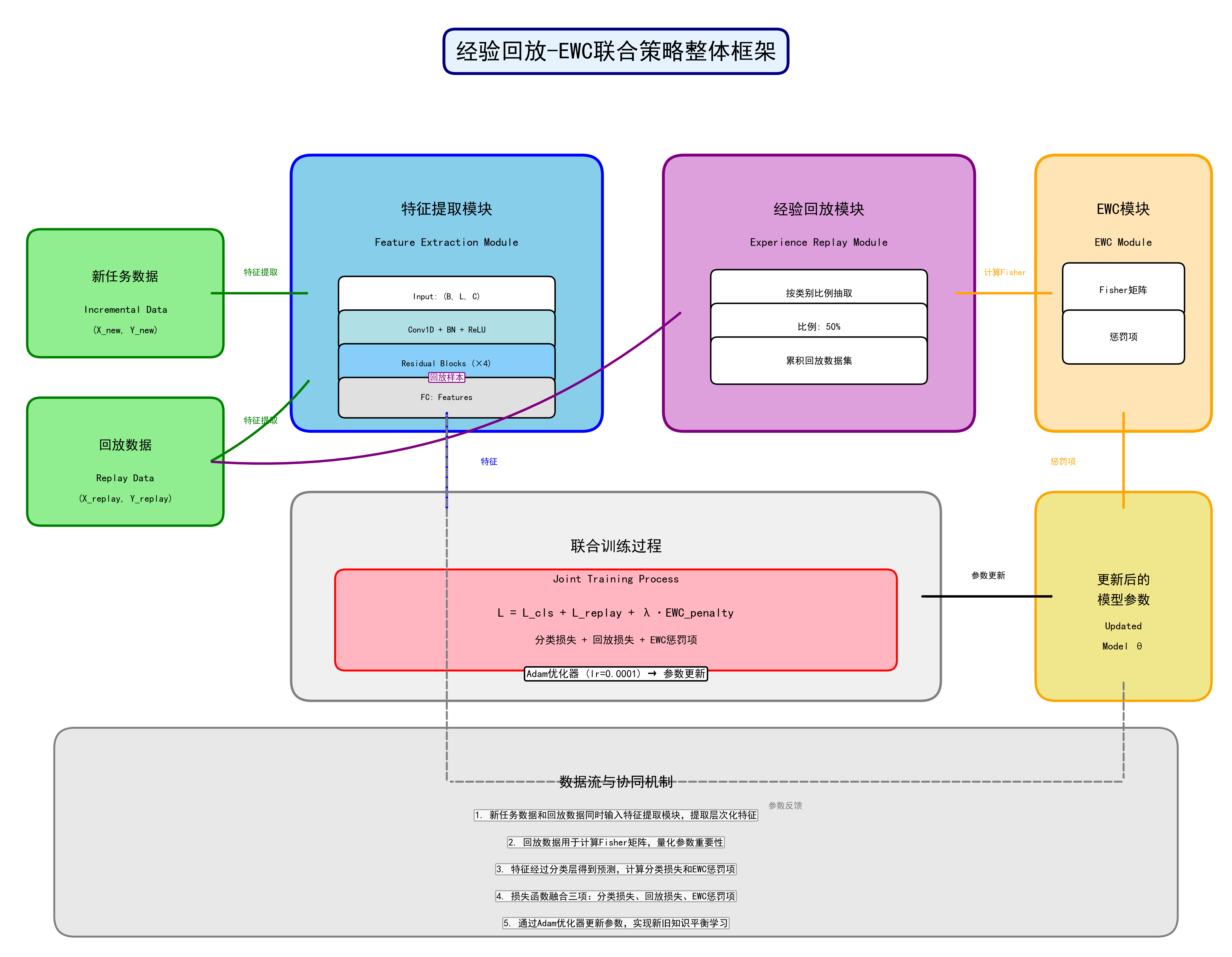
本文提出的解决方案：基于经验回放（Experience Replay）+ 弹性权重巩固（Elastic Weight Consolidation, EWC）的联合策略，让AI系统像人类一样，在学习新知识的同时不忘旧知识。

---

二、项目背景：核电站故障诊断的现实需求

2.1 核电站故障诊断的复杂性

核电站是一个极其复杂的系统，包含：

• 反应堆系统：核反应堆、控制棒、冷却系统

• 蒸汽系统：蒸汽发生器、主蒸汽管道、安全阀

• 给水系统：给水管道、给水泵、给水流量控制

• 安全系统：高压安注系统、压力安全系统

每个系统都可能发生多种故障，例如：

1. 主蒸汽管道破裂：可能导致反应堆失压，是严重事故

1. 冷却剂管道破口：会导致冷却剂流失，可能引发堆芯熔毁

1. 蒸汽发生器传热管破裂（SGTR）：会导致一回路和二回路之间的泄漏

1. 给水流量丧失：会导致蒸汽发生器干涸

1. 掉棒事故：控制棒意外掉落，导致反应性异常

1. 主泵卡轴：主循环泵故障，影响冷却剂循环

1. 安全阀误开启：压力安全系统故障

1. 高压安注系统意外投入：安全系统误动作

2.2 数据特点

本项目使用的数据来自核电站仿真系统，每个故障类型包含：

• 多工况数据：不同功率水平、不同严重程度

• 时序数据：每个样本是时间序列，包含多个传感器读数

• 高维特征：每个时间步包含多个物理参数（压力、温度、流量等）

数据格式：

• 初始数据集：10种故障类型，每种包含多个工况的CSV文件

• 增量数据集：分阶段新增的故障类型

---

三、核心技术原理深度解析

3.1 灾难性遗忘的数学本质

要理解如何解决灾难性遗忘，首先需要理解它的数学本质。

假设我们有一个神经网络模型 f_\\theta(x)，参数为 \\theta。在任务A上训练后，我们得到最优参数 \\theta_A\^：

\\theta_A\^\* = \\arg\\min_\\theta \\mathcal{L}A(\\theta)

其中 \\mathcal{L}A(\\theta) 是任务A上的损失函数。

当我们在任务B上继续训练时，目标是：

\\theta_B\^\* = \\arg\\min_\\theta \\mathcal{L}B(\\theta)

问题在于：如果直接优化 \\mathcal{L}B(\\theta)，参数会从 \\theta_A\^ 移动到 \\theta_B\^，导致模型在任务A上的性能急剧下降。

3.2 经验回放（Experience Replay）机制

核心思想：在学习新任务时，同时回顾旧任务的样本。

实现方式：

1. 在训练初始任务时，保存一部分代表性样本到回放缓冲区（Replay Buffer）

1. 在训练新任务时，从回放缓冲区中采样旧样本，与新样本混合训练

数学表达：

\\mathcal{L}{total} = \\mathcal{L}{new}(\\theta) + \\alpha \\cdot \\mathcal{L}{replay}(\\theta)

其中：

• \\mathcal{L}{new}(\\theta) 是新任务的损失

• \\mathcal{L}{replay}(\\theta) 是回放样本的损失

• \\alpha 是平衡系数

优势：

• 简单直观，易于实现

• 不需要修改网络结构

• 效果显著

局限性：

• 需要存储历史样本（内存开销）

• 回放样本的选择策略影响性能

• 对于大规模数据，回放缓冲区可能不够大

3.3 弹性权重巩固（EWC）机制

核心思想：通过Fisher信息矩阵量化每个参数对旧任务的重要性，对重要参数施加约束，防止其过度偏离最优值。

Fisher信息矩阵：

F_i = \\mathbb{E}{x \\sim p(x\|y), y \\sim p(y)} \\left\[ \\left( \\frac{\\partial \\log p(y\|x, \\theta)}{\\partial \\theta_i} \\right)\^2 \\right\]

Fisher信息矩阵 F_i 衡量参数 \\theta_i 对模型输出的敏感度。F_i 越大，说明 \\theta_i 对任务越重要。

EWC损失函数：

\\mathcal{L}{EWC}(\\theta) = \\mathcal{L}{new}(\\theta) + \\frac{\\lambda}{2} \\sum_i F_i (\\theta_i - \\theta_i\^)\^2

其中：

• \\theta_i\^ 是旧任务的最优参数

• F_i 是参数 \\theta_i 的Fisher信息

• \\lambda 是正则化系数（控制约束强度）

物理意义：

• 如果 F_i 很大（参数重要），则 (\\theta_i - \\theta_i\^)\^2 的惩罚很大，参数不能偏离太远

• 如果 F_i 很小（参数不重要），则允许参数自由调整

优势：

• 不需要存储原始数据，只需要存储Fisher信息矩阵和最优参数

• 理论基础扎实

• 内存效率高

局限性：

• 假设参数空间是二次的（可能不够准确）

• Fisher信息矩阵的计算需要额外开销

• 对于多任务场景，需要累积多个Fisher矩阵

3.4 联合策略：Replay + EWC

为什么联合使用？

1. 互补性：

• Replay提供显式的旧任务样本，让模型直接"看到"旧数据

• EWC提供隐式的参数约束，防止参数过度偏离

1. 双重防护：

• Replay：数据层面的防护

• EWC：参数层面的防护

1. 鲁棒性：

• 即使回放样本选择不当，EWC仍能提供保护

• 即使EWC的Fisher估计不准确，Replay仍能发挥作用

联合损失函数：

\\mathcal{L}{total} = \\mathcal{L}{replay}(\\theta) + \\mathcal{L}{new}(\\theta) + \\lambda{EWC} \\cdot \\mathcal{L}{EWC}(\\theta)

---

四、网络架构设计：ResNet1D详解

4.1 为什么选择ResNet1D？

一维时序数据的特点：

• 核电站传感器数据是时间序列

• 每个时间步包含多个特征（压力、温度、流量等）

• 需要捕捉时序依赖关系

ResNet的优势：

1. 残差连接：解决深层网络的梯度消失问题

1. 批归一化：加速训练，提高稳定性

1. 层次化特征提取：从局部特征到全局特征

4.2 ResNet1D架构详解

输入格式：

• 形状：(batch_size, sequence_length, num_features)

• 例如：(64, 90, 50) 表示64个样本，每个样本90个时间步，每个时间步50个特征

网络结构：

输入 (B, L, C)

↓

转置 (B, C, L) # Conv1d需要通道在前

↓

Conv1d(k=7, s=2) + BN + ReLU

↓

MaxPool1d(k=3, s=2)

↓

Layer1: 2个残差块，64通道

↓

Layer2: 2个残差块，128通道，stride=2

↓

Layer3: 2个残差块，256通道，stride=2

↓

Layer4: 2个残差块，512通道，stride=2

↓

AdaptiveAvgPool1d(1) # 全局平均池化

↓

Flatten

↓

Linear(512, num_classes)

↓

输出 (B, num_classes)

残差块结构：

class ResidualBlock1D(nn.Module):

def init(self, in_channels, out_channels, stride=1):

第一个卷积：可能改变通道数和尺寸

self.conv1 = nn.Conv1d(in_channels, out_channels,

kernel_size=3, stride=stride, padding=1)

self.bn1 = nn.BatchNorm1d(out_channels)

第二个卷积：保持通道数和尺寸

self.conv2 = nn.Conv1d(out_channels, out_channels,

kernel_size=3, stride=1, padding=1)

self.bn2 = nn.BatchNorm1d(out_channels)

下采样层（如果需要）

if stride != 1 or in_channels != out_channels:

self.downsample = nn.Sequential(

nn.Conv1d(in_channels, out_channels,

kernel_size=1, stride=stride),

nn.BatchNorm1d(out_channels)

)

def forward(self, x):

identity = x

out = self.conv1(x)

out = self.bn1(out)

out = F.relu(out)

out = self.conv2(out)

out = self.bn2(out)

残差连接

if self.downsample is not None:

identity = self.downsample(x)

out += identity # 关键：残差连接

out = F.relu(out)

return out

关键设计点：

1. 滑动窗口：将长时序数据切分成固定长度的窗口（如90个时间步）

1. 动态输出层：在增量学习时，扩展分类层以适应新类别数

1. 特征提取器共享：所有任务共享特征提取层，只扩展分类层

---

五、完整实现代码解析

5.1 数据加载与预处理

滑动窗口函数：

def Slidingwindow(dataX, STEPS=10):

"""

将长时序数据切分成固定长度的窗口

输入: dataX shape (T, F) - T个时间步，F个特征

输出: X shape (T-STEPS+1, STEPS, F) - 多个窗口

"""

X = []

for i in range(dataX.shape[0] - STEPS):

X.append(dataX[i:i + STEPS, :])

return np.array(X, dtype=np.float32)

数据加载函数：

def load_data(data_path, class_mapping, steps=90, test_split=0.2):

"""

从指定路径加载数据，自动识别类别

参数:

data_path: 数据根目录

class_mapping: 类别名称到ID的映射

steps: 滑动窗口长度

test_split: 测试集比例

返回:

X_tensor: 特征张量 (N, steps, features)

Y_tensor: 标签张量 (N,)

train_indices: 训练集索引

test_indices: 测试集索引

class_names: 类别名称列表

"""

X = []

Y = []

class_names = []

遍历每个类别文件夹

for class_name in os.listdir(data_path):

if class_name in class_mapping:

class_names.append(class_name)

class_path = os.path.join(data_path, class_name)

遍历该类别的所有CSV文件

for csv_file in os.listdir(class_path):

csv_path = os.path.join(class_path, csv_file)

try:

data = pd.read_csv(csv_path, encoding='gbk')

if data.shape[0] < steps:

continue

滑动窗口切分

x = Slidingwindow(data.values, STEPS=steps)

X.append(x)

Y.append(np.array([class_mapping[class_name]] * x.shape[0]))

except Exception as e:

print(f"读取文件 {csv_path} 时出错: {e}")

合并所有数据

X = np.concatenate(X, axis=0)

Y = np.concatenate(Y, axis=0)

转换为PyTorch张量

X_tensor = torch.tensor(X, dtype=torch.float32)

Y_tensor = torch.tensor(Y, dtype=torch.long)

划分训练集和测试集

dataset_size = len(X_tensor)

indices = list(range(dataset_size))

split = int(np.floor(test_split * dataset_size))

np.random.shuffle(indices)

train_indices, test_indices = indices[split:], indices[:split]

return X_tensor, Y_tensor, train_indices, test_indices, class_names

5.2 回放样本选择策略

按比例选择回放样本：

def select_replay_samples_by_ratio(X, Y, indices, ratio=0.5):

"""

每类按固定比例抽取样本作为回放样本

参数:

X: 特征（未使用，保持接口一致性）

Y: 标签

indices: 候选样本索引

ratio: 抽取比例（0~1）

返回:

replay_indices: 回放样本索引列表

"""

replay_indices = []

unique_classes = torch.unique(Y[indices])

for cls in unique_classes:

找到该类在候选集中的所有索引

class_indices = [idx for idx in indices if Y[idx] == cls]

class_total = len(class_indices)

按比例计算需要抽取的数量

num_samples = max(1, int(class_total * ratio))

num_samples = min(num_samples, class_total)

不放回抽样

if num_samples < class_total:

sampled = np.random.choice(class_indices, num_samples, replace=False)

else:

sampled = class_indices

replay_indices.extend(sampled)

return replay_indices

为什么选择这个策略？

• 简单有效：不需要复杂的采样算法

• 类别平衡：每个类别都按相同比例抽取，保持类别平衡

• 可扩展：随着类别数增加，回放样本库也会增长

5.3 EWC实现详解

EWC类实现：

class EWC:

def init(self, model, dataloader, device, lambda_ewc=10000):

self.model = model

self.dataloader = dataloader

self.device = device

self.lambda_ewc = lambda_ewc

获取所有可训练参数

self.params = {n: p for n, p in self.model.named_parameters()

if p.requires_grad}

初始化Fisher信息矩阵

self.fisher = {n: torch.zeros_like(p.data, device=self.device)

for n, p in self.params.items()}

计算Fisher信息矩阵

self._compute_fisher()

保存旧参数（当前最优参数）

self.old_params = {n: p.clone().detach().to(self.device)

for n, p in self.params.items()}

def _compute_fisher(self):

"""计算Fisher信息矩阵"""

original_mode = self.model.training

self.model.eval()

criterion = nn.CrossEntropyLoss()

计算总样本数（用于归一化）

total_samples = 0

for inputs, _ in self.dataloader:

total_samples += inputs.size(0)

累加梯度平方

for inputs, targets in self.dataloader:

inputs, targets = inputs.to(self.device), targets.to(self.device)

self.model.zero_grad()

outputs = self.model(inputs)

loss = criterion(outputs, targets)

loss.backward()

累加每个参数的梯度平方

for n, p in self.params.items():

if p.grad is not None:

self.fisher[n] += (p.grad ** 2) / total_samples

恢复模型原始模式

self.model.train(original_mode)

def penalty(self):

"""计算EWC惩罚项"""

loss = 0.0

for n, p in self.params.items():

确保所有张量在同一设备

fisher = self.fisher[n]

old_param = self.old_params[n]

EWC惩罚：F_i * (θ_i - θ_i^*)^2

loss += (fisher * (p - old_param) ** 2).sum()

return self.lambda_ewc * loss / 2

关键点解析：

1. Fisher信息矩阵计算：

• 在旧任务的最优参数上计算

• 使用回放数据（或旧任务数据）

• 对梯度平方求平均（归一化）

1. 惩罚项计算：

• 对每个参数计算 (θ_i - θ_i\^)\^2

• 乘以对应的Fisher信息 F_i

• 求和后乘以正则化系数 \\lambda_{EWC}

1. 参数更新：

• 在训练新任务时，总损失 = 分类损失 + EWC惩罚

• 通过反向传播更新参数

• 重要参数（F_i大）的更新幅度会被限制

5.4 增量训练流程

核心训练函数：

def train_with_replay_and_incremental(

model, replay_loader, incremental_loader,

test_loader, history_test_loader, incremental_test_loader,

ewc, epochs=100, lr=0.0001

):

"""

使用Replay+EWC进行增量训练

参数:

model: 待训练的模型

replay_loader: 回放数据加载器（包含所有历史回放样本）

incremental_loader: 增量数据加载器（当前阶段的新数据）

test_loader: 合并测试集加载器

history_test_loader: 历史类别测试集加载器

incremental_test_loader: 增量类别测试集加载器

ewc: EWC对象

epochs: 训练轮数

lr: 学习率

"""

model.train()

optimizer = optim.Adam(model.parameters(), lr=lr)

criterion = nn.CrossEntropyLoss()

train_losses = []

test_accuracies = []

initial_test_accuracies = []

incremental_test_accuracies = []

for epoch in range(epochs):

running_loss = 0.0

correct = 0

total = 0

创建迭代器

replay_iter = iter(replay_loader)

incre

incremental_iter = iter(incremental_loader)

确定最大迭代次数

max_iter = max(len(replay_loader), len(incremental_loader))

for i in range(max_iter):

处理回放数据

try:

replay_inputs, replay_targets = next(replay_iter)

replay_inputs, replay_targets = replay_inputs.to(device), replay_targets.to(device)

optimizer.zero_grad()

replay_outputs = model(replay_inputs)

replay_loss = criterion(replay_outputs, replay_targets)

添加EWC惩罚

replay_penalty = ewc.penalty()

replay_loss = replay_loss + replay_penalty

replay_loss.backward()

optimizer.step()

running_loss += replay_loss.item()

, predicted = replay_outputs.max(1)

total += replay_targets.size(0)

correct += predicted.eq(replay_targets).sum().item()

except StopIteration:

replay_iter = iter(replay_loader)

处理增量数据

try:

inc_inputs, inc_targets = next(incremental_iter)

inc_inputs, inc_targets = inc_inputs.to(device), inc_targets.to(device)

optimizer.zero_grad()

inc_outputs = model(inc_inputs)

inc_loss = criterion(inc_outputs, inc_targets)

添加EWC惩罚

inc_penalty = ewc.penalty()

inc_loss = inc_loss + inc_penalty

inc_loss.backward()

optimizer.step()

running_loss += inc_loss.item()

, predicted = inc_outputs.max(1)

total += inc_targets.size(0)

correct += predicted.eq(inc_targets).sum().item()

except StopIteration:

incremental_iter = iter(incremental_loader)

计算平均损失

epoch_loss = running_loss / (2 * max_iter)

epoch_acc = correct / total

train_losses.append(epoch_loss)

评估模型

test_accuracy, , = test_model(model, test_loader)

initial_test_accuracy, , = test_model(model, history_test_loader)

incremental_test_accuracy, , = test_model(model, incremental_test_loader)

test_accuracies.append(test_accuracy)

initial_test_accuracies.append(initial_test_accuracy)

incremental_test_accuracies.append(incremental_test_accuracy)

print(f'Epoch {epoch + 1}/{epochs}, 训练Loss: {epoch_loss:.4f}, 训练Acc: {epoch_acc:.4f}')

print(f' 合并测试集Accuracy: {test_accuracy:.4f}')

print(f' 历史类别测试集Accuracy: {initial_test_accuracy:.4f}')

print(f' 当前增量类别测试集Accuracy: {incremental_test_accuracy:.4f}')

return model, train_losses, test_accuracies, initial_test_accuracies, incremental_test_accuracies

**训练流程的关键点**：

1. **混合训练**：每个epoch中，回放数据和增量数据交替训练

2. **双重损失**：回放数据和增量数据都添加EWC惩罚

3. **多维度评估**：同时评估合并准确率、历史准确率、增量准确率

5.5 主函数：完整的增量学习流程

**主函数核心逻辑**：

ython

def main():

超参数设置

batch_size = 64

initial_epochs = 100

learning_rate = 0.001

steps = 90 # 时间序列长度

replay_ratio = 0.5 # 回放样本比例

incremental_epochs = 100

lambda_ewc = 10000 # EWC正则化系数

1. 获取初始类别映射

initial_classid = get_initial_class_mapping(INITIAL_DATA_PATH)

2. 获取增量学习阶段

incremental_stages, incremental_class_mappings = get_incremental_stages(INCREMENTAL_STAGES_PATH)

3. 分配类别ID

incremental_class_mappings, combined_class_mappings = assign_class_ids(

initial_classid, incremental_class_mappings

)

4. 加载初始数据并训练初始模型

X_initial, Y_initial, train_indices_initial, test_indices_initial, _ = load_data(

INITIAL_DATA_PATH, initial_classid, steps=steps

)

model = create_resnet_model(input_size=X_initial.shape[2],

num_classes=len(initial_classid)).to(device)

训练初始模型

model, initial_train_losses, initial_test_accuracies = train_model(

model, initial_train_loader, initial_test_loader,

epochs=initial_epochs, lr=learning_rate

)

5. 选择初始回放样本

replay_indices_initial = select_replay_samples_by_ratio(

X_initial, Y_initial, train_indices_initial, ra