day39模型的可视化和推理@浙大疏锦行

主要针对隐藏层神经元的个数进行了修改

python 复制代码

# 实验 1: 原始配置 (隐藏层神经元 = 10)
print("=== 实验 1: 原始配置 (Hidden Size = 10) ===")
model_base = MLP(input_size=4, hidden_size=10, output_size=3).to(device)
time_base, acc_base, losses_base = train_and_evaluate(model_base, learning_rate=0.01, num_epochs=10000, desc="Base Model")
print(f"Base Model - Time: {time_base:.2f}s, Accuracy: {acc_base*100:.2f}%")

# 实验 2: 增加隐藏层神经元 (隐藏层神经元 = 50)
print("\n=== 实验 2: 增加隐藏层神经元 (Hidden Size = 50) ===")
model_large = MLP(input_size=4, hidden_size=50, output_size=3).to(device)
time_large, acc_large, losses_large = train_and_evaluate(model_large, learning_rate=0.01, num_epochs=10000, desc="Large Model")
print(f"Large Model - Time: {time_large:.2f}s, Accuracy: {acc_large*100:.2f}%")

# 实验 3: 减少隐藏层神经元 (隐藏层神经元 = 4)
print("\n=== 实验 3: 减少隐藏层神经元 (Hidden Size = 4) ===")
model_small = MLP(input_size=4, hidden_size=4, output_size=3).to(device)
time_small, acc_small, losses_small = train_and_evaluate(model_small, learning_rate=0.01, num_epochs=10000, desc="Small Model")
print(f"Small Model - Time: {time_small:.2f}s, Accuracy: {acc_small*100:.2f}%")

markdown 复制代码

=== 实验 1: 原始配置 (Hidden Size = 10) ===
Base Model: 10000/10000 [00:12<00:00, 780.84epoch/s, Loss=0.0943]
Base Model: 10000/10000 [00:12<00:00, 780.84epoch/s, Loss=0.0943]
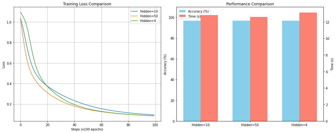
Base Model - Time: 12.81s, Accuracy: 96.67%

=== 实验 2: 增加隐藏层神经元 (Hidden Size = 50) ===
Large Model:  10000/10000 [00:12<00:00, 793.83epoch/s, Loss=0.0857]
Large Model:  10000/10000 [00:12<00:00, 793.83epoch/s, Loss=0.0857]
Large Model - Time: 12.60s, Accuracy: 96.67%

=== 实验 3: 减少隐藏层神经元 (Hidden Size = 4) ===
Small Model:  10000/10000 [00:13<00:00, 761.09epoch/s, Loss=0.0849]
Small Model - Time: 13.14s, Accuracy: 96.67%

可视化

python 复制代码

# 可视化对比
plt.figure(figsize=(15, 6))

# Loss Curve
plt.subplot(1, 2, 1)
plt.plot(losses_base, label='Hidden=10')
plt.plot(losses_large, label='Hidden=50')
plt.plot(losses_small, label='Hidden=4')
plt.xlabel('Steps (x100 epochs)')
plt.ylabel('Loss')
plt.title('Training Loss Comparison')
plt.legend()
plt.grid(True)

# Accuracy and Time Bar Chart
plt.subplot(1, 2, 2)
models = ['Hidden=10', 'Hidden=50', 'Hidden=4']
accs = [acc_base * 100, acc_large * 100, acc_small * 100] # Convert to percentage
times = [time_base, time_large, time_small]

x = np.arange(len(models))
width = 0.35

ax1 = plt.gca()
ax2 = ax1.twinx()

bars1 = ax1.bar(x - width/2, accs, width, label='Accuracy (%)', color='skyblue')
bars2 = ax2.bar(x + width/2, times, width, label='Time (s)', color='salmon')

ax1.set_ylabel('Accuracy (%)')
ax2.set_ylabel('Time (s)')
ax1.set_ylim(0, 110) # Accuracy 0-100+
ax1.set_xticks(x)
ax1.set_xticklabels(models)
plt.title('Performance Comparison')

# Add legends
lines1, labels1 = ax1.get_legend_handles_labels()
lines2, labels2 = ax2.get_legend_handles_labels()
ax1.legend(lines1 + lines2, labels1 + labels2, loc='upper left')

plt.tight_layout()
plt.show()

@浙大疏锦行