1. 引言
圆柱立铣刀的容屑槽是其关键结构之一,几何要素的正确设计直接影响刀具的切削性能和排屑能力。容屑槽的主要几何要素包括刀刃曲线、槽宽曲线和芯厚回转面,这些要素由前角 γ \gamma γ、芯厚半径 c c c、螺旋角 β \beta β和槽宽角 α \alpha α等参数定义。通过建立准确的数学模型,可以对这些几何要素进行仿真分析,从而优化刀具设计。本文基于圆弧投影法建立容屑槽的数学模型,并使用Python进行三维可视化仿真,为容屑槽的刃磨工艺优化提供理论依据。
2. 数学基础与几何模型
2.1 坐标系定义
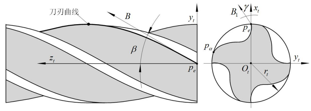
建立刀具坐标系 { O t ; x t , y t , z t } \{O_t;x_t,y_t,z_t\} {Ot;xt,yt,zt},其中 x t x_t xt轴和 y t y_t yt轴位于刀具的端面, x t x_t xt轴正半轴穿过刀尖点 p e p_e pe,原点 O t O_t Ot位于工件圆的中心, z t z_t zt轴沿刀轴指向刀具内部。该坐标系是分析容屑槽几何要素的基础。
2.2 几何参数定义
螺旋角 β \beta β定义为轴向平面刀刃曲线在 p e p_e pe点处的切向量 B B B与 z t z_t zt轴之间的夹角,满足:
B = 0 sin β cos β T B=0\\quad\\sin\\beta\\quad\\cos\\beta^{\mathrm{T}} B=0sinβcosβT
前角 γ \gamma γ定义为端平面 p e p_e pe点处 x t x_t xt轴与前刀面在 p e p_e pe点的切向量 B 1 B_1 B1之间的夹角,满足:
B 1 = cos γ − sin γ 0 T B_1=\\cos\\gamma\\quad-\\sin\\gamma\\quad 0^{\mathrm{T}} B1=cosγ−sinγ0T
刀尖点 p e p_e pe的坐标为:
p e = r t 0 0 T p_e=r_t\\quad 0\\quad 0^{\mathrm{T}} pe=rt00T
其中 r t r_t rt为刀具半径。
2.3 几何要素参数方程
刀刃曲线由刀尖点 p e p_e pe绕 z t z_t zt轴做螺旋运动形成,参数方程为:
R t ( ω ) ( ω t ) = r t cos ω e r t sin ω e r t ω e cot β R_t^{(\omega)}(\omega_t) = \begin{bmatrix} r_t \cos\omega_e \\ r_t \sin\omega_e \\ r_t \omega_e \cot\beta \end{bmatrix} Rt(ω)(ωt)=⎣⎡rtcosωertsinωertωecotβ⎦⎤
槽宽曲线由容屑槽尾部 p a p_a pa点绕 z t z_t zt轴做螺旋运动形成,参数方程为:
R ( ω ) ( ω e ) = r t cos ( ω e − α ) r t sin ( ω e − α ) r t ω e cot β R^{(\omega)}(\omega_e) = \begin{bmatrix} r_t \cos(\omega_e - \alpha) \\ r_t \sin(\omega_e - \alpha) \\ r_t \omega_e \cot\beta \end{bmatrix} R(ω)(ωe)=⎣⎡rtcos(ωe−α)rtsin(ωe−α)rtωecotβ⎦⎤
芯厚回转面是芯厚半径所在的圆沿 z t z_t zt轴做直线运动形成的圆柱面,参数方程为:
R t ( ω ) ( h e , ω e ) = c cos ω e c sin ω e h t R_t^{(\omega)}(h_e,\omega_e) = \begin{bmatrix} c\cos\omega_e \\ c\sin\omega_e \\ h_t \end{bmatrix} Rt(ω)(he,ωe)=⎣⎡ccosωecsinωeht⎦⎤
其中 ω e \omega_e ωe为旋转角度参数, h t h_t ht为沿 z t z_t zt轴的移动距离。
3. Python仿真实现
3.1 三维几何要素仿真
以下代码独立实现了圆柱立铣刀容屑槽几何要素的三维仿真,包括刀刃曲线、槽宽曲线和芯厚回转面的可视化:
python
import numpy as np
import matplotlib.pyplot as plt
from mpl_toolkits.mplot3d import Axes3D

# 设置几何参数
r_t = 2.0  # 刀具半径 (mm)
c = 2.0    # 芯厚半径 (mm)
beta = 30  # 螺旋角 (度)
alpha = 75  # 槽宽角 (度)

# 转换为弧度
beta_rad = np.deg2rad(beta)
alpha_rad = np.deg2rad(alpha)

# 生成刀刃曲线 (螺旋线)
omega_e = np.linspace(0, 4 * np.pi, 200)
x_edge = r_t * np.cos(omega_e)
y_edge = r_t * np.sin(omega_e)
z_edge = r_t * omega_e * np.cos(beta_rad) / np.sin(beta_rad)

# 生成槽宽曲线
x_flute = r_t * np.cos(omega_e - alpha_rad)
y_flute = r_t * np.sin(omega_e - alpha_rad)
z_flute = r_t * omega_e * np.cos(beta_rad) / np.sin(beta_rad)

# 生成芯厚回转面
z_vals = np.linspace(0, np.max(z_edge), 50)
theta = np.linspace(0, 2 * np.pi, 50)
Z, Theta = np.meshgrid(z_vals, theta)
x_core = c * np.cos(Theta)
y_core = c * np.sin(Theta)
z_core = Z

# 创建三维图形
fig = plt.figure(figsize=(12, 8))
ax = fig.add_subplot(111, projection='3d')

# 绘制芯厚回转面
ax.plot_surface(x_core, y_core, z_core, alpha=0.3, color='lightblue',
                edgecolor='gray', linewidth=0.5, rstride=2, cstride=2)

# 绘制刀刃曲线
ax.plot(x_edge, y_edge, z_edge, 'r-', linewidth=2, label='Cutting edge curve')

# 绘制槽宽曲线
ax.plot(x_flute, y_flute, z_flute, 'b-', linewidth=2, label='Flute width curve')

# 标注关键点
p_e = [r_t, 0, 0]
p_a = [r_t * np.cos(-alpha_rad), r_t * np.sin(-alpha_rad), 0]

ax.scatter([p_e[0]], [p_e[1]], [p_e[2]], color='red', s=50, marker='o')
ax.text(p_e[0], p_e[1], p_e[2], ' p_e', fontsize=10, color='red')

ax.scatter([p_a[0]], [p_a[1]], [p_a[2]], color='blue', s=50, marker='o')
ax.text(p_a[0], p_a[1], p_a[2], ' p_a', fontsize=10, color='blue')

# 添加标注
ax.text(0, 0, 9, 'Core surface', fontsize=10, color='darkblue',
        horizontalalignment='center', verticalalignment='center')

# 设置图形属性
ax.set_xlabel('X (mm)', fontsize=12, labelpad=10)
ax.set_ylabel('Y (mm)', fontsize=12, labelpad=10)
ax.set_zlabel('Z (mm)', fontsize=12, labelpad=10)
ax.set_title('Geometric Elements of Cylindrical End Mill Flute', fontsize=14, pad=20)
ax.legend(loc='upper right')
ax.view_init(elev=20, azim=45)
ax.grid(True, alpha=0.3)

# 添加参数信息
param_text = f'$r_t$ = {r_t} mm\n$c$ = {c} mm\n$\\beta$ = {beta}°\n$\\alpha$ = {alpha}°'
ax.text2D(0.02, 0.98, param_text, transform=ax.transAxes, fontsize=10,
          verticalalignment='top', bbox=dict(boxstyle='round', facecolor='wheat', alpha=0.8))

plt.tight_layout()
plt.savefig('end_mill_3d_view.png', dpi=300, bbox_inches='tight')
plt.show()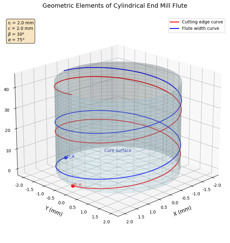
3.2 端面投影图仿真
以下代码独立实现了圆柱立铣刀端面投影图的仿真,展示了前角 γ \gamma γ和槽宽角 α \alpha α的定义:
python
import numpy as np
import matplotlib.pyplot as plt

# 设置几何参数
r_t = 2.0  # 刀具半径 (mm)
c = 2.0    # 芯厚半径 (mm)
gamma = 10  # 前角 (度)
alpha = 75  # 槽宽角 (度)

# 转换为弧度
gamma_rad = np.deg2rad(gamma)
alpha_rad = np.deg2rad(alpha)

# 创建图形
fig, ax = plt.subplots(figsize=(8, 8))

# 绘制刀具外圆
theta_circle = np.linspace(0, 2*np.pi, 100)
ax.plot(r_t * np.cos(theta_circle), r_t * np.sin(theta_circle),
        'k-', linewidth=1.5, label='Tool contour')

# 绘制芯厚圆
ax.plot(c * np.cos(theta_circle), c * np.sin(theta_circle),
        'k--', linewidth=1, label='Core circle')

# 标记刀尖点 p_e
p_e = [r_t, 0]
ax.plot(p_e[0], p_e[1], 'ro', markersize=8, label='p_e (cutting edge)')
ax.text(p_e[0]+0.1, p_e[1], 'p_e', fontsize=10, color='red')

# 标记槽宽起点 p_a
p_a = [r_t * np.cos(-alpha_rad), r_t * np.sin(-alpha_rad)]
ax.plot(p_a[0], p_a[1], 'bo', markersize=8, label='p_a (flute start)')
ax.text(p_a[0]-0.2, p_a[1]-0.2, 'p_a', fontsize=10, color='blue')

# 绘制前角参考线
scale = 1.5
B1_x = scale * np.cos(gamma_rad)
B1_y = scale * -np.sin(gamma_rad)
ax.arrow(p_e[0], p_e[1], B1_x, B1_y,
         head_width=0.1, head_length=0.1, fc='red', ec='red', linewidth=1.5)

# 绘制x轴参考线
ax.arrow(0, 0, scale, 0,
         head_width=0.1, head_length=0.1, fc='black', ec='black', linewidth=1.5)

# 绘制前角γ标注
gamma_arc_radius = 0.6
theta_gamma = np.linspace(0, gamma_rad, 50)
ax.plot(gamma_arc_radius * np.cos(theta_gamma),
        gamma_arc_radius * np.sin(theta_gamma),
        'r-', linewidth=1.5)
ax.text(gamma_arc_radius * np.cos(gamma_rad/2) * 1.1,
        gamma_arc_radius * np.sin(gamma_rad/2) * 1.1,
        f'$\gamma$={gamma}°', fontsize=10, color='red')

# 绘制槽宽角α
alpha_arc_radius = 0.8
theta_alpha = np.linspace(-alpha_rad, 0, 50)
ax.plot(alpha_arc_radius * np.cos(theta_alpha),
        alpha_arc_radius * np.sin(theta_alpha),
        'b-', linewidth=1.5)
ax.text(alpha_arc_radius * np.cos(-alpha_rad/2) * 1.1,
        alpha_arc_radius * np.sin(-alpha_rad/2) * 1.1,
        f'$\\alpha$={alpha}°', fontsize=10, color='blue')

# 设置图形属性
ax.set_aspect('equal')
ax.grid(True, alpha=0.3)
ax.set_xlabel('X (mm)', fontsize=12)
ax.set_ylabel('Y (mm)', fontsize=12)
ax.set_title('End Face View of Cylindrical End Mill', fontsize=14)
ax.set_xlim(-2.5, 2.5)
ax.set_ylim(-2.5, 2.5)
ax.legend(loc='upper right', fontsize=10)

plt.tight_layout()
plt.savefig('end_face_view.png', dpi=300, bbox_inches='tight')
plt.show()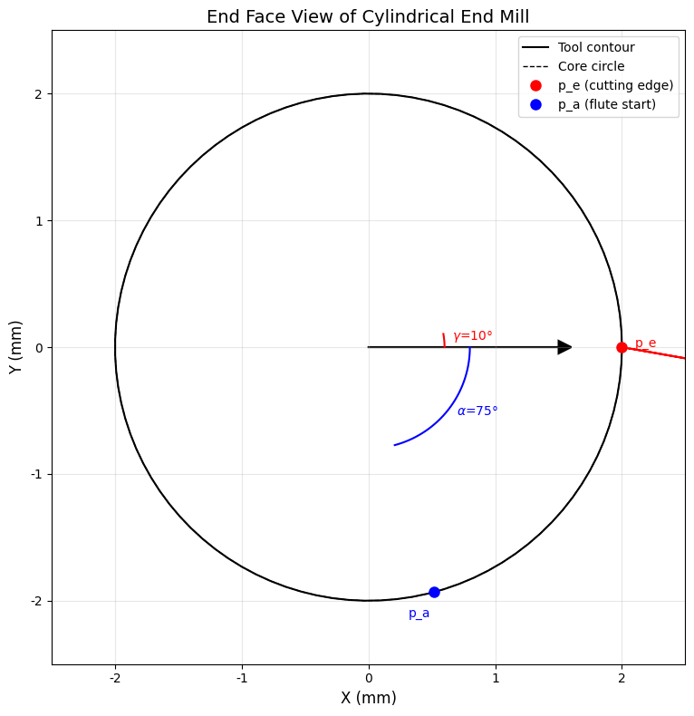
3.3 几何参数计算与分析
以下代码独立实现了容屑槽关键几何参数的计算,包括前刀面法向量、曲线长度和螺旋升程等:
python
import numpy as np

def calculate_geometric_parameters(r_t, beta, gamma, c, alpha):
    """
    计算圆柱立铣刀容屑槽的关键几何参数

    参数:
    r_t: 刀具半径 (mm)
    beta: 螺旋角 (度)
    gamma: 前角 (度)
    c: 芯厚半径 (mm)
    alpha: 槽宽角 (度)

    返回:
    包含所有计算结果的字典
    """
    # 转换为弧度
    beta_rad = np.deg2rad(beta)
    gamma_rad = np.deg2rad(gamma)
    alpha_rad = np.deg2rad(alpha)

    # 计算刀尖点处的切向量B和B1
    B = np.array([0, np.sin(beta_rad), np.cos(beta_rad)])
    B1 = np.array([np.cos(gamma_rad), -np.sin(gamma_rad), 0])

    # 计算前刀面在刀尖点处的单位法向量
    cross_product = np.cross(B, B1)
    N_t = cross_product / np.linalg.norm(cross_product)

    # 计算螺旋升程 (导程)
    lead = 2 * np.pi * r_t / np.tan(beta_rad)

    # 计算芯厚比
    core_ratio = c / r_t

    # 计算槽宽对应的弧长
    arc_length = r_t * alpha_rad

    # 计算刀刃曲线螺旋参数
    helix_parameter = r_t * np.tan(beta_rad)

    results = {
        'tool_radius': r_t,
        'core_radius': c,
        'helix_angle': beta,
        'rake_angle': gamma,
        'flute_width_angle': alpha,
        'cutting_edge_vector': B,
        'rake_face_vector': B1,
        'normal_vector': N_t,
        'lead': lead,
        'core_ratio': core_ratio,
        'arc_length': arc_length,
        'helix_parameter': helix_parameter
    }

    return results

# 示例计算
parameters = calculate_geometric_parameters(
    r_t=2.0, beta=30, gamma=10, c=2.0, alpha=75
)

# 输出计算结果
print("圆柱立铣刀几何参数计算结果:")
print("=" * 50)
print(f"刀具半径 r_t: {parameters['tool_radius']} mm")
print(f"芯厚半径 c: {parameters['core_radius']} mm")
print(f"螺旋角 β: {parameters['helix_angle']}°")
print(f"前角 γ: {parameters['rake_angle']}°")
print(f"槽宽角 α: {parameters['flute_width_angle']}°")
print(f"螺旋升程 (导程): {parameters['lead']:.2f} mm")
print(f"芯厚比 (c/r_t): {parameters['core_ratio']:.3f}")
print(f"槽宽对应弧长: {parameters['arc_length']:.3f} mm")
print(f"刀刃切向量 B: [{parameters['cutting_edge_vector'][0]:.3f}, "
      f"{parameters['cutting_edge_vector'][1]:.3f}, "
      f"{parameters['cutting_edge_vector'][2]:.3f}]")
print(f"前刀面切向量 B1: [{parameters['rake_face_vector'][0]:.3f}, "
      f"{parameters['rake_face_vector'][1]:.3f}, "
      f"{parameters['rake_face_vector'][2]:.3f}]")
print(f"前刀面法向量 N_t: [{parameters['normal_vector'][0]:.3f}, "
      f"{parameters['normal_vector'][1]:.3f}, "
      f"{parameters['normal_vector'][2]:.3f}]")

# 参数敏感性分析示例
print("\n参数敏感性分析:")
print("=" * 50)
helix_angles = [20, 30, 40, 50]
for beta_test in helix_angles:
    test_params = calculate_geometric_parameters(2.0, beta_test, 10, 2.0, 75)
    print(f"螺旋角 {beta_test}°: 导程 = {test_params['lead']:.2f} mm, "
          f"螺旋参数 = {test_params['helix_parameter']:.3f}")
4. 仿真结果分析
仿真结果显示,圆柱立铣刀的容屑槽几何要素具有以下特征:
-
刀刃曲线 :呈现规则的螺旋线形状,螺旋角 β \beta β决定了曲线的陡峭程度。当 β \beta β增大时,螺旋线变得更加陡峭,导程减小。
-
槽宽曲线 :与刀刃曲线平行但存在相位差 α \alpha α,表示容屑槽的宽度分布。槽宽角 α \alpha α直接影响容屑槽的容积和排屑能力。
-
芯厚回转面 :形成刀具的芯部支撑结构,芯厚半径 c c c与刀具半径 r t r_t rt的比例影响刀具的刚度和强度。
-
前角 γ \gamma γ的影响 :在端面视图中,前角 γ \gamma γ决定了前刀面的倾斜程度,直接影响切削刃的锋利程度和切屑流动方向。
-
几何参数关系 :螺旋升程 L L L与螺旋角 β \beta β的关系为 L = 2 π r t / tan β L = 2\pi r_t / \tan\beta L=2πrt/tanβ,表明在固定刀具半径下,螺旋角越大,导程越小,螺旋线越紧密。
5. 工程应用与优化
基于上述几何模型,可以进一步优化容屑槽设计:
-
刃磨工艺优化:通过调整砂轮位姿,精确控制容屑槽的几何参数,确保加工质量。
-
切削性能预测:根据几何参数计算切削力、切屑形状和刀具寿命,指导刀具选型。
-
参数优化设计 :通过调整 β \beta β、 γ \gamma γ、 c c c、 α \alpha α等参数,平衡刀具的刚度、锋利度和排屑能力。
-
制造误差分析:分析几何参数偏差对切削性能的影响,制定合理的制造公差。
6. 结论
本文建立了圆柱立铣刀容屑槽几何要素的完整数学模型,通过Python实现了三维可视化仿真和参数计算。仿真结果直观展示了刀刃曲线、槽宽曲线和芯厚回转面的空间几何关系,为容屑槽的设计和刃磨工艺优化提供了理论依据。通过调整几何参数,可以优化刀具的切削性能和排屑能力,满足不同加工条件的需求。未来的研究可以进一步考虑容屑槽的刃磨动力学和加工误差分析,提高刀具的制造精度和使用寿命。