小目标检测：PinwheelConv详解

前言

最近找到的小目标检测论文很多都是红外领域的，需要处理热成像信息，还有些用分割方法做红外小目标检测。这些都与我的可见光目标检测任务不匹配，加上开源代码少，导致最近一段研究进展困难。今天要学习的是风车卷积PConv，虽然也是做红外小目标检测的，但也能用到我们的任务当中。

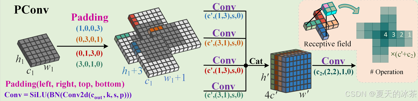
今天要学习的是一个很简单的一个结构PConv，相信大家对其很熟悉，去年的时候很多的yolo改进，还有b站的讲解视频都在说这个。作者发现卷积神经网络通常采用标准卷积，未能考虑到红外小目标像素的空间特性，因此提出了一个风车形卷积PConv，可在骨干网络底层中替换标准卷积，PConv更符合弱小目标的像素高斯空间分布，增强了特征提取能力，显著扩大了感受野，且仅引入了极小的参数增加。

当然，对于这个模块是否适合普通的小目标，我们要经过实验才能知道，因为除了符合红外特征空间分布以外，其还具有扩大感受野的功效。

论文地址：Pinwheel-shaped Convolution and Scale-based Dynamic Loss for Infrared Small Target Detection

代码：https://github.com/JN-Yang/PConv-SDloss-Data

PConv结构

python 复制代码

import torch
import torch.nn as nn
from ultralytics.nn.modules import Conv, C2f

class PConv(nn.Module):
    ''' Pinwheel-shaped Convolution using the Asymmetric Padding method. '''
    def __init__(self, c1, c2, k, s, p=None):
        super().__init__()
        # self.k = k
        p = [(k, 0, 1, 0), (0, k, 0, 1), (0, 1, k, 0), (1, 0, 0, k)]
        self.pad = [nn.ZeroPad2d(padding=(p[g])) for g in range(4)]
        self.cw = Conv(c1, c2 // 4, (1, k), s=s, p=0)
        self.ch = Conv(c1, c2 // 4, (k, 1), s=s, p=0)
        self.cat = Conv(c2, c2, 2, s=1, p=0)

    def forward(self, x):
        yw0 = self.cw(self.pad[0](x))
        yw1 = self.cw(self.pad[1](x))
        yh0 = self.ch(self.pad[2](x))
        yh1 = self.ch(self.pad[3](x))
        return self.cat(torch.cat([yw0, yw1, yh0, yh1], dim=1))

我们从代码讲起：

p = [(k, 0, 1, 0), (0, k, 0, 1), (0, 1, k, 0), (1, 0, 0, k)]

这定义了4种不同的填充方式，例如p[0]: (k, 0, 1, 0) → 左填充k个像素，上填充1个像素；p[1]: (0, k, 0, 1) → 右填充k个像素，下填充1个像素；p[2]: (0, 1, k, 0) → 右填充1个像素，上填充k个像素；p[3]: (1, 0, 0, k) → 左填充1个像素，下填充k个像素。

然后通过两个方向卷积，水平方向1×k卷积核，垂直方向k×1卷积核。形成了四个分支，最后通过一个2x2小卷积进行融合，这个2×2的小卷积核可以在相邻的4个通道组之间进行信息交换。

前面已经有过四个方向的特征提取了，所以在这里只用做轻量的融合了，我思考过这里为什么不用1x1卷积呢，作者说的是风车卷积（PConv）可以与标准卷积层互换，并作为通道注意力机制，用于分析不同卷积方向的贡献。

但我觉得还有就是1x1卷积只能做通道混合，没有空间信息，而2x2卷积有最小的空间感受野，能兼顾通道和空间，这里又学到了一个点。

APC2f模块

python 复制代码

class APBottleneck(nn.Module):
    """Asymmetric Padding bottleneck."""
    def __init__(self, c1, c2, shortcut=True, g=1, k=(3, 3), e=0.5):
        """Initializes a bottleneck module with given input/output channels, shortcut option, group, kernels, and
        expansion.
        """
        super().__init__()
        c_ = int(c2 * e)  # hidden channels
        p = [(2, 0, 2, 0), (0, 2, 0, 2), (0, 2, 2, 0), (2, 0, 0, 2)]
        self.pad = [nn.ZeroPad2d(padding=(p[g])) for g in range(4)]
        self.cv1 = Conv(c1, c_ // 4, k[0], 1, p=0)
        self.cv2 = Conv(c_, c2, k[1], 1, g=g)
        self.add = shortcut and c1 == c2

    def forward(self, x):
        """'forward()' applies the YOLO FPN to input data."""
        return x + self.cv2((torch.cat([self.cv1(self.pad[g](x)) for g in range(4)], 1))) if self.add else self.cv2(
            (torch.cat([self.cv1(self.pad[g](x)) for g in range(4)], 1)))

class APC2f(C2f):
    def __init__(self, c1: int, c2: int, n: int = 1, shortcut: bool = False, g: int = 1, e: float = 0.5):
        super(APC2f, self).__init__(c1, c2, n, shortcut, g, e)
        self.m = nn.ModuleList(
            APBottleneck(self.c, self.c, shortcut, g, k=((3, 3), (3, 3)), e=1.0) for _ in range(n))

论文里面没用看到这个结构，作者提供的配置文件也将PConv替换了前两层的Conv，但作者在代码中又提供了这个APC2f。

这里就是定义了4种不同的2像素非对称填充，整体的思路与PConv相似，不过没有方向型卷积，仅做了拼接的处理，下面我们做实验也将其添加上。

消融实验

因为我对红外的小目标暂时还不感什么兴趣，所以这里我就还是采用PConv+APC2f的组合在yolov8上做改进，然后进行消融实验，下面是详细的配置文件：

python 复制代码

# Parameters
nc: 80 # number of classes
scales: # model compound scaling constants, i.e. 'model=yolov8n.yaml' will call yolov8.yaml with scale 'n'
  # [depth, width, max_channels]
  n: [0.33, 0.25, 1024] # YOLOv8n summary: 129 layers, 3157200 parameters, 3157184 gradients, 8.9 GFLOPS
  s: [0.33, 0.50, 1024] # YOLOv8s summary: 129 layers, 11166560 parameters, 11166544 gradients, 28.8 GFLOPS
  m: [0.67, 0.75, 768] # YOLOv8m summary: 169 layers, 25902640 parameters, 25902624 gradients, 79.3 GFLOPS
  l: [1.00, 1.00, 512] # YOLOv8l summary: 209 layers, 43691520 parameters, 43691504 gradients, 165.7 GFLOPS
  x: [1.00, 1.25, 512] # YOLOv8x summary: 209 layers, 68229648 parameters, 68229632 gradients, 258.5 GFLOPS


# YOLOv8.0 backbone
backbone:
  # [from, repeats, module, args]
  - [-1, 1, PConv, [64, 4, 2]] # 0-P1/2
  - [-1, 1, PConv, [128, 4, 2]] # 1-P2/4
  - [-1, 3, APC2f, [128, True]]
  - [-1, 1, Conv, [256, 3, 2]] # 3-P3/8
  - [-1, 6, C2f, [256, True]]
  - [-1, 1, Conv, [512, 3, 2]] # 5-P4/16
  - [-1, 6, APC2f, [512, True]]
  - [-1, 1, Conv, [1024, 3, 2]] # 7-P5/32
  - [-1, 3, APC2f, [1024, True]]
  - [-1, 1, SPPF, [1024, 5]] # 9

# YOLOv8.0-p2 head
head:
  - [-1, 1, nn.Upsample, [None, 2, "nearest"]]
  - [[-1, 6], 1, Concat, [1]] # cat backbone P4
  - [-1, 3, C2f, [512]] # 12

  - [-1, 1, nn.Upsample, [None, 2, "nearest"]]
  - [[-1, 4], 1, Concat, [1]] # cat backbone P3
  - [-1, 3, C2f, [256]] # 15 (P3/8-small)

  - [-1, 1, nn.Upsample, [None, 2, "nearest"]]
  - [[-1, 2], 1, Concat, [1]] # cat backbone P2
  - [-1, 3, C2f, [128]] # 18 (P2/4-xsmall)

  - [-1, 1, Conv, [128, 3, 2]]
  - [[-1, 15], 1, Concat, [1]] # cat head P3
  - [-1, 3, APC2f, [256]] # 21 (P3/8-small)

  - [-1, 1, Conv, [256, 3, 2]]
  - [[-1, 12], 1, Concat, [1]] # cat head P4
  - [-1, 3, APC2f, [512]] # 24 (P4/16-medium)

  - [-1, 1, Conv, [512, 3, 2]]
  - [[-1, 9], 1, Concat, [1]] # cat head P5
  - [-1, 3, APC2f, [1024]] # 27 (P5/32-large)

  - [[18, 21, 24, 27], 1, Detect, [nc]] # Detect(P2, P3, P4, P5)

精度 (P): 0.0103

召回率 (R): 0.0143

mAP50 (IoU=0.5时的平均精度): 0.00476

mAP50-95 (IoU=0.5到0.95的平均精度): 0.00145