介绍
亚马逊销售数据集生动地展现了现代商业的一个横截面,揭示了消费者行为和订单履行的趋势。在本笔记本中,我们将探索数据的各个方面------从清理和可视化到开发一个预测交易总额的模型。
python
# Import necessary libraries and set configurations
import warnings
warnings.filterwarnings('ignore')

import numpy as np
import pandas as pd

import matplotlib
matplotlib.use('Agg')  # Ensure we use the Agg backend
import matplotlib.pyplot as plt
%matplotlib inline

import seaborn as sns
sns.set(style="whitegrid")

# Print a quick version check (uncomment if needed)
# print('Pandas version:', pd.__version__)
# print('NumPy version:', np.__version__)
python
# Load the Amazon sales dataset
df = pd.read_csv('/Amazon.csv', encoding='ascii', delimiter=',')

# Display the first few rows to verify the data loaded correctly
print('Dataset Shape:', df.shape)
df.head()Dataset Shape: (100000, 20)|---|------------|------------|------------|---------------|-----------|---------------------|-----------------|------------|----------|-----------|----------|-------|--------------|-------------|------------------|-------------|-------------|-------|---------------|-----------|
| | OrderID | OrderDate | CustomerID | CustomerName | ProductID | ProductName | Category | Brand | Quantity | UnitPrice | Discount | Tax | ShippingCost | TotalAmount | PaymentMethod | OrderStatus | City | State | Country | SellerID |
| 0 | ORD0000001 | 2023-01-31 | CUST001504 | Vihaan Sharma | P00014 | Drone Mini | Books | BrightLux | 3 | 106.59 | 0.00 | 0.00 | 0.09 | 319.86 | Debit Card | Delivered | Washington | DC | India | SELL01967 |
| 1 | ORD0000002 | 2023-12-30 | CUST000178 | Pooja Kumar | P00040 | Microphone | Home & Kitchen | UrbanStyle | 1 | 251.37 | 0.05 | 19.10 | 1.74 | 259.64 | Amazon Pay | Delivered | Fort Worth | TX | United States | SELL01298 |
| 2 | ORD0000003 | 2022-05-10 | CUST047516 | Sneha Singh | P00044 | Power Bank 20000mAh | Clothing | UrbanStyle | 3 | 35.03 | 0.10 | 7.57 | 5.91 | 108.06 | Debit Card | Delivered | Austin | TX | United States | SELL00908 |
| 3 | ORD0000004 | 2023-07-18 | CUST030059 | Vihaan Reddy | P00041 | Webcam Full HD | Home & Kitchen | Zenith | 5 | 33.58 | 0.15 | 11.42 | 5.53 | 159.66 | Cash on Delivery | Delivered | Charlotte | NC | India | SELL01164 |
| 4 | ORD0000005 | 2023-02-04 | CUST048677 | Aditya Kapoor | P00029 | T-Shirt | Clothing | KiddoFun | 2 | 515.64 | 0.25 | 38.67 | 9.23 | 821.36 | Credit Card | Cancelled | San Antonio | TX | Canada | SELL01411 |
数据加载与预处理
在本节中,我们将对数据进行清理,并执行预处理步骤。请注意,"OrderDate"列原本是字符串类型,将被转换为日期时间对象,但在格式不符合预期的情况下,这可能会成为产生错误的原因。如果您遇到日期转换问题,请确保在 pd.to_datetime 函数中的格式参数被正确指定。
python
# Convert OrderDate to datetime format
df['OrderDate'] = pd.to_datetime(df['OrderDate'], errors='coerce')

# Check for missing values in the dataset
missing_values = df.isnull().sum()
print('Missing values in each column:')
print(missing_values)

# (Optional) Drop rows or fill missing values if any - here we simply show the counts
# df.dropna(inplace=True)  # Uncomment if you wish to drop missing values entirely

# Display info to verify data types
df.info()Missing values in each column:
OrderID 0
OrderDate 0
CustomerID 0
CustomerName 0
ProductID 0
ProductName 0
Category 0
Brand 0
Quantity 0
UnitPrice 0
Discount 0
Tax 0
ShippingCost 0
TotalAmount 0
PaymentMethod 0
OrderStatus 0
City 0
State 0
Country 0
SellerID 0
dtype: int64
<class 'pandas.core.frame.DataFrame'>
RangeIndex: 100000 entries, 0 to 99999
Data columns (total 20 columns):
# Column Non-Null Count Dtype
--- ------ -------------- -----
0 OrderID 100000 non-null object
1 OrderDate 100000 non-null datetime64[ns]
2 CustomerID 100000 non-null object
3 CustomerName 100000 non-null object
4 ProductID 100000 non-null object
5 ProductName 100000 non-null object
6 Category 100000 non-null object
7 Brand 100000 non-null object
8 Quantity 100000 non-null int64
9 UnitPrice 100000 non-null float64
10 Discount 100000 non-null float64
11 Tax 100000 non-null float64
12 ShippingCost 100000 non-null float64
13 TotalAmount 100000 non-null float64
14 PaymentMethod 100000 non-null object
15 OrderStatus 100000 non-null object
16 City 100000 non-null object
17 State 100000 non-null object
18 Country 100000 non-null object
19 SellerID 100000 non-null object
dtypes: datetime64[ns](1), float64(5), int64(1), object(13)
memory usage: 15.3+ MB探索性数据分析
在这里,我们对数据集进行了多种可视化处理,包括相关性热图、配对图以及分布图表等。这有助于在开发任何预测模型之前,增强我们对数据的直观理解。
我们采用了多种可视化方法,包括热图、直方图、关联图、箱形图等等,以全面呈现情况。
python
# Select numeric columns for correlation analysis
numeric_df = df.select_dtypes(include=[np.number])

# Only plot if we have at least four numeric columns
if numeric_df.shape[1] >= 4:
    plt.figure(figsize=(10, 8))
    corr_matrix = numeric_df.corr()
    sns.heatmap(corr_matrix, annot=True, cmap='coolwarm', fmt='.2f')
    plt.title('Correlation Heatmap of Numeric Features')
    plt.show()
else:
    print('Not enough numeric columns for a correlation heatmap.')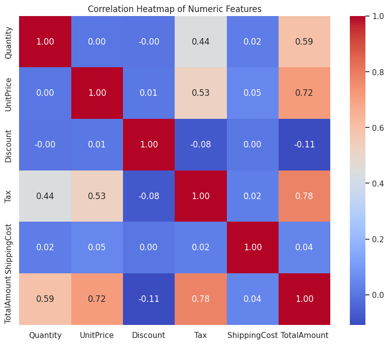
python
# Create a pair plot for selected numerical features
# Using a subset of features that are believed to impact the TotalAmount
pairplot_cols = ['Quantity', 'UnitPrice', 'Discount', 'Tax', 'ShippingCost', 'TotalAmount']
if set(pairplot_cols).issubset(df.columns):
    sns.pairplot(df[pairplot_cols].dropna())
    plt.suptitle('Pair Plot for Selected Numerical Features', y=1.02)
    plt.show()
else:
    print('Some of the required columns for pair plot are missing.')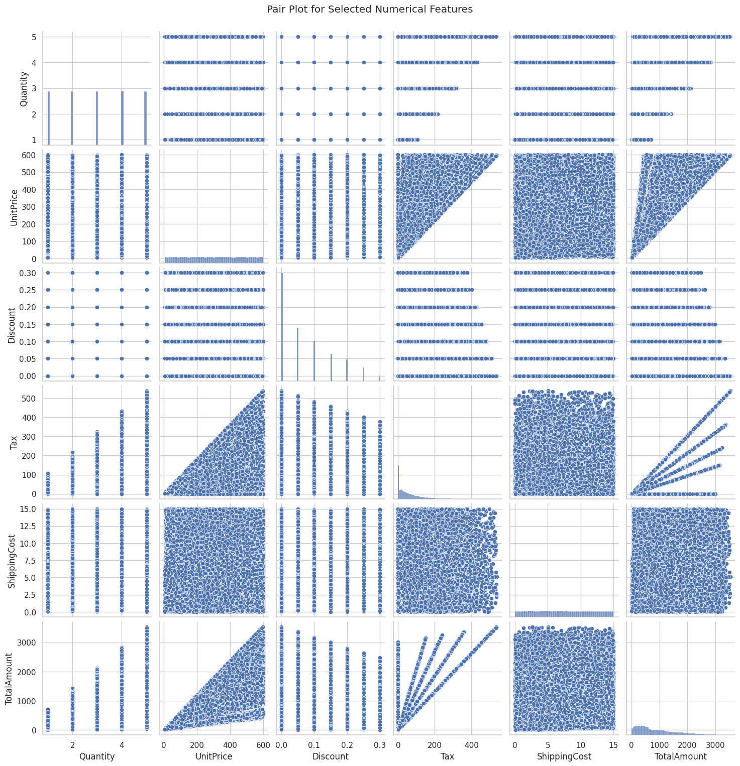
python
# Plot a histogram for the TotalAmount to get an idea of its distribution
plt.figure(figsize=(8, 5))
sns.histplot(df['TotalAmount'].dropna(), bins=30, kde=True, color='skyblue')
plt.title('Distribution of TotalAmount')
plt.xlabel('TotalAmount')
plt.ylabel('Frequency')
plt.show()
python
# Plot a count plot for PaymentMethod to see the frequency of each method
plt.figure(figsize=(8, 5))
sns.countplot(data=df, x='PaymentMethod', palette='viridis')
plt.title('Count Plot of Payment Methods')
plt.xlabel('Payment Method')
plt.ylabel('Count')
plt.xticks(rotation=45)
plt.show()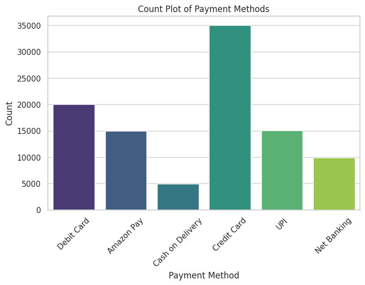
python
# Box plot to understand the distribution of UnitPrice
plt.figure(figsize=(8, 5))
sns.boxplot(data=df, y='UnitPrice', color='lightgreen')
plt.title('Box Plot of UnitPrice')
plt.ylabel('UnitPrice')
plt.show()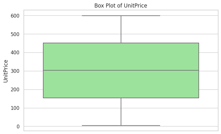
python
# Boxen plot to visualize the Discount across different Categories
plt.figure(figsize=(10, 6))
sns.boxenplot(data=df, x='Category', y='Discount', palette='Pastel1')
plt.title('Discount Distribution by Category')
plt.xlabel('Category')
plt.ylabel('Discount')
plt.xticks(rotation=45)
plt.show()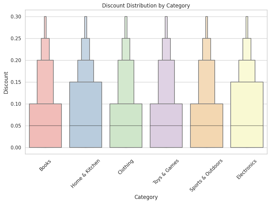
python
# Violin plot to compare ShippingCost distribution among Payment Methods
plt.figure(figsize=(10, 6))
sns.violinplot(data=df, x='PaymentMethod', y='ShippingCost', palette='muted')
plt.title('ShippingCost Distribution by PaymentMethod')
plt.xlabel('PaymentMethod')
plt.ylabel('ShippingCost')
plt.xticks(rotation=45)
plt.show()
python
# Strip plot to show TotalAmount variation across different OrderStatus values
plt.figure(figsize=(10, 6))
sns.stripplot(data=df, x='OrderStatus', y='TotalAmount', jitter=True, palette='Spectral')
plt.title('TotalAmount by OrderStatus')
plt.xlabel('OrderStatus')
plt.ylabel('TotalAmount')
plt.xticks(rotation=45)
plt.show()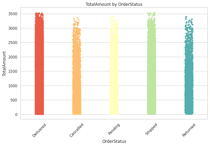
预测建模
在本节中,我们试图预测订单的总金额。我们选择了那些为数值型且可能对总销售额产生影响的特征:数量、单价、折扣、税费以及运费。
由于"总金额"是一个连续变量,所以我们采用回归模型。在回归分析中,准确性最好通过 R² 分数来衡量。如果遇到与特征编码或缺失数据相关的错误,请务必进行适当的预处理。
python
from sklearn.model_selection import train_test_split
from sklearn.linear_model import LinearRegression
from sklearn.metrics import r2_score

# Define features and target
feature_cols = ['Quantity', 'UnitPrice', 'Discount', 'Tax', 'ShippingCost']
target_col = 'TotalAmount'

# Drop rows with missing values in the features/target columns
model_df = df[feature_cols + [target_col]].dropna()

# Split the data into training and testing sets
X = model_df[feature_cols]
y = model_df[target_col]

X_train, X_test, y_train, y_test = train_test_split(X, y, test_size=0.2, random_state=42)

# Initialize and train the linear regression model
lr = LinearRegression()
lr.fit(X_train, y_train)

# Predict on the test set
y_pred = lr.predict(X_test)

# Calculate R^2 score for prediction accuracy
r2 = r2_score(y_test, y_pred)
print('R² score on the test set:', r2)

# A side note: In regression tasks, we measure prediction quality with metrics like R². Unlike classification, accuracy score is not applicable.R² score on the test set: 0.9095060550803165总结与未来工作
这篇内容对亚马逊销售数据集进行了全面的分析,从数据清洗和预处理开始,接着运用多种可视化技术进行了深入的探索性数据分析,最后还开发了一个能够预测总金额的回归模型。
多种可视化图表(热图、配对图、直方图、箱线图和细线图)揭示了数据中的关键模式,而预测模型也达到了一定的 R² 值,从而为订单总额的可预测性提供了初步的见解。
未来分析的方向可能包括:
对其他功能进行了试验,包括从日期字段中提取的定制功能(例如,月份或星期几)。
尝试使用更高级的建模技术,如集成方法或梯度提升,以提高预测的准确性。
进行更详细的错误分析,以了解并解决异常值或数据质量问题。