引言
在精密磨削加工中,砂轮的几何轮廓直接影响加工精度和表面质量。本文基于参数化建模方法,推导了具有复杂轮廓的砂轮的数学模型,并提供了完整的Python实现。该模型能够精确描述包含圆弧过渡段和锥面段的砂轮轮廓,为后续的包络计算和加工仿真奠定基础。
砂轮轮廓的数学模型
砂轮坐标系定义
砂轮坐标系 Og−XgYgZgO_g-X_gY_gZ_gOg−XgYgZg 定义如下:
- 原点 OgO_gOg 位于砂轮端面中心
- ZgZ_gZg 轴垂直于砂轮端面
- XgX_gXg 和 YgY_gYg 轴位于端面内
参数化表面方程
砂轮轮廓面上任一点 WWW 在砂轮坐标系中的齐次坐标表示为:
Wg=(xg(h,θ)yg(h,θ)zg(h,θ)1)=(R(h)cosθR(h)sinθh1),h∈0,H,θ∈0,2π W_{g} = \begin{pmatrix} x_{g}(h,\theta) \\ y_{g}(h,\theta) \\ z_{g}(h,\theta) \\ 1 \end{pmatrix} = \begin{pmatrix} R(h)\cos\theta \\ R(h)\sin\theta \\ h \\ 1 \end{pmatrix}, \quad h \in 0, H, \theta \in 0, 2\\pi Wg= xg(h,θ)yg(h,θ)zg(h,θ)1 = R(h)cosθR(h)sinθh1 ,h∈0,H,θ∈0,2π
其中:
- hhh:砂轮轮廓高度(轴向位置变量)
- θ\thetaθ:旋转角
- R(h)R(h)R(h):半径函数
- HHH:砂轮宽度
半径函数的分段定义
根据 hhh 的不同取值范围,半径函数 R(h)R(h)R(h) 分段定义为:
R(h)={R−Rwl+Rwl2−(Rwl−h)2,h∈0,hLR(hL)−(h−hL)tanκ,h∈hL,H−hrR(hL)−hmtanκ−Rwrcosκ+Rwr2−(Rwr−H+h)2,h∈H−hr,H R(h) = \begin{cases} R - R_{wl} + \sqrt{R_{wl}^{2} - (R_{wl} - h)^{2}}, & h \in 0, h_{L} \\ R(h_{L}) - (h - h_{L}) \tan \kappa, & h \in h_{L}, H - h_{r} \\ R(h_{L}) - h_{m} \tan \kappa - R_{wr} \cos \kappa + \sqrt{R_{wr}^{2} - (R_{wr} - H + h)^{2}}, & h \in H - h_{r}, H \end{cases} R(h)=⎩ ⎨ ⎧R−Rwl+Rwl2−(Rwl−h)2 ,R(hL)−(h−hL)tanκ,R(hL)−hmtanκ−Rwrcosκ+Rwr2−(Rwr−H+h)2 ,h∈0,hLh∈hL,H−hrh∈H−hr,H
相关几何参数:
- RRR:砂轮基本半径
- RwlR_{wl}Rwl:左侧轮廓圆角半径
- RwrR_{wr}Rwr:右侧轮廓圆角半径
- hLh_{L}hL:左侧切点的轴向位置
- hrh_{r}hr:右侧切点的轴向位置
- hmh_{m}hm:锥面段的轴向长度
- κ\kappaκ:砂轮锥角
角度参数与几何关系
圆弧对应的中心角与砂轮锥角的关系:
{α0=π2+κα1=π2−κ \begin{cases} \alpha_{0} = \frac{\pi}{2} + \kappa \\ \alpha_{1} = \frac{\pi}{2} - \kappa \end{cases} {α0=2π+κα1=2π−κ
左侧圆弧 CACACA 上 hhh 与 αAC\alpha_{AC}αAC 的显式关系:
h(αAC)=2Rwlsin2αAC2,αAC∈0,α0 h(\alpha_{AC}) = 2R_{wl} \sin^{2} \frac{\alpha_{AC}}{2}, \quad \alpha_{AC} \in 0, \\alpha_{0} h(αAC)=2Rwlsin22αAC,αAC∈0,α0
右侧圆弧 BDBDBD 的几何关系:
{hr=Rwrtanα12hm=H−hL−hrh(αBD)=H−2Rwrsin2αBD2,αBD∈0,α1 \begin{cases} h_{r} = R_{wr} \tan \frac{\alpha_{1}}{2} \\ h_{m} = H - h_{L} - h_{r} \\ h(\alpha_{BD}) = H - 2R_{wr} \sin^{2} \frac{\alpha_{BD}}{2}, \quad \alpha_{BD} \in 0, \\alpha_{1} \end{cases} ⎩ ⎨ ⎧hr=Rwrtan2α1hm=H−hL−hrh(αBD)=H−2Rwrsin22αBD,αBD∈0,α1
完整的Python实现
代码实现:砂轮轮廓计算类
python
import numpy as np
import matplotlib.pyplot as plt
from matplotlib import cm
from mpl_toolkits.mplot3d import Axes3D

# 设置中文字体支持
plt.rcParams['font.sans-serif'] = ['SimHei', 'Microsoft YaHei', 'DejaVu Sans']
plt.rcParams['axes.unicode_minus'] = False

class GrindingWheelProfile:
    """砂轮轮廓计算与绘制类"""

    def __init__(self,
                 R: float = 50.0,
                 R_wl: float = 5.0,
                 R_wr: float = 5.0,
                 H: float = 30.0,
                 kappa: float = 15.0):
        """
        初始化砂轮参数

        参数:
        R: 砂轮基本半径 (mm)
        R_wl: 左侧轮廓圆角半径 (mm)
        R_wr: 右侧轮廓圆角半径 (mm)
        H: 砂轮宽度 (mm)
        kappa: 砂轮锥角 (度)
        """
        # 基本参数
        self.R = R
        self.R_wl = R_wl
        self.R_wr = R_wr
        self.H = H
        self.kappa = np.deg2rad(kappa)  # 转换为弧度

        # 计算相关几何参数
        self._calculate_parameters()

    def _calculate_parameters(self):
        """计算几何参数"""
        # 公式(2-3): 计算角度参数
        self.alpha_0 = np.pi/2 + self.kappa  # 左侧圆弧最大中心角
        self.alpha_1 = np.pi/2 - self.kappa  # 右侧圆弧最大中心角

        # 公式(2-5): 计算左侧切点A的轴向位置h_L
        self.h_L = 2 * self.R_wl * (np.sin(self.alpha_0/2)**2)

        # 公式(2-6): 计算右侧切点B的轴向位置h_r和锥面段长度h_m
        self.h_r = self.R_wr * np.tan(self.alpha_1/2)
        self.h_m = self.H - self.h_L - self.h_r

        # 计算h=h_L处的半径值
        self.R_hL = self.R - self.R_wl + np.sqrt(self.R_wl**2 - (self.R_wl - self.h_L)**2)

    def R_h(self, h: np.ndarray) -> np.ndarray:
        """
        公式(2-2): 半径函数分段计算

        参数:
        h: 轴向位置数组

        返回:
        R: 对应半径数组
        """
        h = np.asarray(h)
        R = np.zeros_like(h)

        # 分段条件
        left_mask = h <= self.h_L  # 左侧圆弧段
        middle_mask = (h > self.h_L) & (h <= self.H - self.h_r)  # 锥面段
        right_mask = h > self.H - self.h_r  # 右侧圆弧段

        # 左侧圆弧段 (0 <= h <= h_L)
        if np.any(left_mask):
            h_left = h[left_mask]
            R[left_mask] = (self.R - self.R_wl +
                           np.sqrt(self.R_wl**2 - (self.R_wl - h_left)**2))

        # 锥面段 (h_L < h <= H - h_r)
        if np.any(middle_mask):
            h_middle = h[middle_mask]
            R[middle_mask] = self.R_hL - (h_middle - self.h_L) * np.tan(self.kappa)

        # 右侧圆弧段 (H - h_r < h <= H)
        if np.any(right_mask):
            h_right = h[right_mask]
            term = (self.R_wr - self.H + h_right)
            R[right_mask] = (self.R_hL - self.h_m * np.tan(self.kappa) -
                            self.R_wr * np.cos(self.kappa) +
                            np.sqrt(self.R_wr**2 - term**2))

        return R

    def parametric_surface(self, n_h: int = 100, n_theta: int = 50) -> tuple:
        """
        生成砂轮三维参数化表面

        参数:
        n_h: 轴向采样点数
        n_theta: 圆周方向采样点数

        返回:
        X, Y, Z: 三维坐标数组
        """
        # 生成参数网格
        h = np.linspace(0, self.H, n_h)
        theta = np.linspace(0, 2*np.pi, n_theta)
        h_grid, theta_grid = np.meshgrid(h, theta, indexing='ij')

        # 计算半径
        R_grid = self.R_h(h_grid)

        # 转换为直角坐标
        X = R_grid * np.cos(theta_grid)
        Y = R_grid * np.sin(theta_grid)
        Z = h_grid

        return X, Y, Z

    def profile_points(self, n_points: int = 500) -> tuple:
        """
        获取砂轮轮廓母线点

        参数:
        n_points: 采样点数

        返回:
        h_points, R_points: 轴向位置和半径数组
        """
        h_points = np.linspace(0, self.H, n_points)
        R_points = self.R_h(h_points)
        return h_points, R_points

    def get_key_points(self) -> dict:
        """
        获取关键特征点

        返回:
        key_points: 关键点字典,包含坐标点和参数
        """
        # 左侧圆弧起点C (h=0)
        C = (0, self.R - self.R_wl)

        # 左侧切点A (h=h_L)
        A = (self.h_L, self.R_hL)

        # 右侧切点B (h=H-h_r)
        h_B = self.H - self.h_r
        R_B = self.R_hL - (h_B - self.h_L) * np.tan(self.kappa)
        B = (h_B, R_B)

        # 右侧圆弧终点D (h=H)
        D = (self.H, self.R_h(np.array([self.H]))[0])

        return {
            'C': C,  # 左侧圆弧起点 (h, R)
            'A': A,  # 左侧切点 (h, R)
            'B': B,  # 右侧切点 (h, R)
            'D': D,  # 右侧圆弧终点 (h, R)
            'h_L': self.h_L,     # 左侧圆弧长度
            'h_r': self.h_r,     # 右侧圆弧长度
            'h_m': self.h_m,     # 锥面段长度
            'R_hL': self.R_hL    # 左侧切点处半径
        }

# 创建砂轮对象
wheel = GrindingWheelProfile(
    R=50.0,      # 基本半径 50mm
    R_wl=5.0,    # 左侧圆角半径 5mm
    R_wr=5.0,    # 右侧圆角半径 5mm
    H=30.0,      # 砂轮宽度 30mm
    kappa=15.0   # 锥角 15度
)

# 打印砂轮参数
print("=" * 50)
print("砂轮参数:")
print("=" * 50)
print(f"基本半径 R = {wheel.R} mm")
print(f"左侧圆角半径 R_wl = {wheel.R_wl} mm")
print(f"右侧圆角半径 R_wr = {wheel.R_wr} mm")
print(f"砂轮宽度 H = {wheel.H} mm")
print(f"锥角 κ = {np.rad2deg(wheel.kappa):.1f}°")
print(f"左侧最大中心角 α₀ = {np.rad2deg(wheel.alpha_0):.1f}°")
print(f"右侧最大中心角 α₁ = {np.rad2deg(wheel.alpha_1):.1f}°")

# 获取关键点并正确打印
key_points = wheel.get_key_points()

print("\n" + "=" * 50)
print("关键点坐标 (h, R):")
print("=" * 50)
for point_name in ['C', 'A', 'B', 'D']:
    h, R = key_points[point_name]
    print(f"点{point_name}: h = {h:.2f} mm, R = {R:.2f} mm")

print("\n" + "=" * 50)
print("特征长度:")
print("=" * 50)
print(f"左侧圆弧长度 h_L = {key_points['h_L']:.2f} mm")
print(f"右侧圆弧长度 h_r = {key_points['h_r']:.2f} mm")
print(f"锥面段长度 h_m = {key_points['h_m']:.2f} mm")
print(f"左侧切点处半径 R_hL = {key_points['R_hL']:.2f} mm")
print("=" * 50)
代码实现:二维轮廓可视化
python
import numpy as np
import matplotlib.pyplot as plt

# 重新定义GrindingWheelProfile类确保独立运行
class GrindingWheelProfile:
    def __init__(self, R=50.0, R_wl=5.0, R_wr=5.0, H=30.0, kappa=15.0):
        self.R = R
        self.R_wl = R_wl
        self.R_wr = R_wr
        self.H = H
        self.kappa = np.deg2rad(kappa)
        self._calculate_parameters()

    def _calculate_parameters(self):
        self.alpha_0 = np.pi/2 + self.kappa
        self.alpha_1 = np.pi/2 - self.kappa
        self.h_L = 2 * self.R_wl * (np.sin(self.alpha_0/2)**2)
        self.h_r = self.R_wr * np.tan(self.alpha_1/2)
        self.h_m = self.H - self.h_L - self.h_r
        self.R_hL = self.R - self.R_wl + np.sqrt(self.R_wl**2 - (self.R_wl - self.h_L)**2)

    def R_h(self, h):
        h = np.asarray(h)
        R = np.zeros_like(h)

        left_mask = h <= self.h_L
        middle_mask = (h > self.h_L) & (h <= self.H - self.h_r)
        right_mask = h > self.H - self.h_r

        if np.any(left_mask):
            h_left = h[left_mask]
            R[left_mask] = self.R - self.R_wl + np.sqrt(self.R_wl**2 - (self.R_wl - h_left)**2)

        if np.any(middle_mask):
            h_middle = h[middle_mask]
            R[middle_mask] = self.R_hL - (h_middle - self.h_L) * np.tan(self.kappa)

        if np.any(right_mask):
            h_right = h[right_mask]
            term = (self.R_wr - self.H + h_right)
            R[right_mask] = (self.R_hL - self.h_m * np.tan(self.kappa) -
                            self.R_wr * np.cos(self.kappa) +
                            np.sqrt(self.R_wr**2 - term**2))

        return R

# 创建砂轮对象
wheel = GrindingWheelProfile(R=50.0, R_wl=5.0, R_wr=5.0, H=30.0, kappa=15.0)

# 获取关键点
h_L = wheel.h_L
h_r = wheel.h_r
R_hL = wheel.R_hL

# 创建图形
fig, ax = plt.subplots(figsize=(10, 6))

# 生成轮廓点
h_points = np.linspace(0, wheel.H, 500)
R_points = wheel.R_h(h_points)

# 绘制轮廓线
ax.plot(h_points, R_points, 'b-', linewidth=2, label='Grinding wheel profile')
ax.plot(h_points, -R_points, 'b--', linewidth=1, alpha=0.5)

# 绘制中心线
ax.axhline(y=0, color='k', linestyle='-', linewidth=0.5, alpha=0.3)

# 计算关键点坐标
C = (0, wheel.R - wheel.R_wl)
A = (h_L, R_hL)
h_B = wheel.H - h_r
R_B = R_hL - (h_B - h_L) * np.tan(wheel.kappa)
B = (h_B, R_B)
D = (wheel.H, wheel.R_h(np.array([wheel.H]))[0])

# 绘制关键点
key_points = {'C': C, 'A': A, 'B': B, 'D': D}
colors = {'C': 'r', 'A': 'g', 'B': 'm', 'D': 'c'}
markers = {'C': 'o', 'A': 's', 'B': '^', 'D': 'v'}

for point_name, (h, R) in key_points.items():
    ax.plot(h, R, f'{colors[point_name]}{markers[point_name]}', markersize=8,
            label=f'Point {point_name}', markeredgecolor='k')

# 绘制不同线段
h_left = np.linspace(0, h_L, 50)
R_left = wheel.R_h(h_left)
ax.plot(h_left, R_left, 'r-', linewidth=1, alpha=0.5, label='Left arc segment')

h_mid = np.linspace(h_L, wheel.H - h_r, 50)
R_mid = wheel.R_h(h_mid)
ax.plot(h_mid, R_mid, 'g-', linewidth=2, alpha=0.7, label='Conical segment')

h_right = np.linspace(wheel.H - h_r, wheel.H, 50)
R_right = wheel.R_h(h_right)
ax.plot(h_right, R_right, 'm-', linewidth=1, alpha=0.5, label='Right arc segment')

# 设置图形属性
ax.set_xlabel('Axial position h (mm)', fontsize=12)
ax.set_ylabel('Radius R(h) (mm)', fontsize=12)
ax.set_title('Grinding Wheel Profile', fontsize=14, fontweight='bold')
ax.grid(True, alpha=0.3)
ax.legend(loc='best')
ax.axis('equal')

# 添加标注
ax.text(0.02, 0.98, f'κ = {np.rad2deg(wheel.kappa):.1f}°',
        transform=ax.transAxes, verticalalignment='top',
        bbox=dict(boxstyle='round', facecolor='wheat', alpha=0.8))

plt.tight_layout()
plt.show()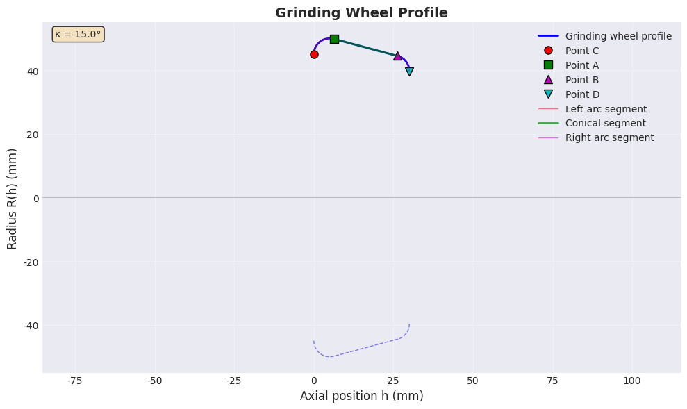
代码实现:三维表面可视化
python
import numpy as np
import matplotlib.pyplot as plt
from matplotlib import cm
from mpl_toolkits.mplot3d import Axes3D

# 重新定义GrindingWheelProfile类确保独立运行
class GrindingWheelProfile:
    def __init__(self, R=50.0, R_wl=5.0, R_wr=5.0, H=30.0, kappa=15.0):
        self.R = R
        self.R_wl = R_wl
        self.R_wr = R_wr
        self.H = H
        self.kappa = np.deg2rad(kappa)
        self._calculate_parameters()

    def _calculate_parameters(self):
        self.alpha_0 = np.pi/2 + self.kappa
        self.alpha_1 = np.pi/2 - self.kappa
        self.h_L = 2 * self.R_wl * (np.sin(self.alpha_0/2)**2)
        self.h_r = self.R_wr * np.tan(self.alpha_1/2)
        self.h_m = self.H - self.h_L - self.h_r
        self.R_hL = self.R - self.R_wl + np.sqrt(self.R_wl**2 - (self.R_wl - self.h_L)**2)

    def R_h(self, h):
        h = np.asarray(h)
        R = np.zeros_like(h)

        left_mask = h <= self.h_L
        middle_mask = (h > self.h_L) & (h <= self.H - self.h_r)
        right_mask = h > self.H - self.h_r

        if np.any(left_mask):
            h_left = h[left_mask]
            R[left_mask] = self.R - self.R_wl + np.sqrt(self.R_wl**2 - (self.R_wl - h_left)**2)

        if np.any(middle_mask):
            h_middle = h[middle_mask]
            R[middle_mask] = self.R_hL - (h_middle - self.h_L) * np.tan(self.kappa)

        if np.any(right_mask):
            h_right = h[right_mask]
            term = (self.R_wr - self.H + h_right)
            R[right_mask] = (self.R_hL - self.h_m * np.tan(self.kappa) -
                            self.R_wr * np.cos(self.kappa) +
                            np.sqrt(self.R_wr**2 - term**2))

        return R

    def parametric_surface(self, n_h=100, n_theta=50):
        h = np.linspace(0, self.H, n_h)
        theta = np.linspace(0, 2*np.pi, n_theta)
        h_grid, theta_grid = np.meshgrid(h, theta, indexing='ij')

        R_grid = self.R_h(h_grid)

        X = R_grid * np.cos(theta_grid)
        Y = R_grid * np.sin(theta_grid)
        Z = h_grid

        return X, Y, Z

# 创建砂轮对象
wheel = GrindingWheelProfile(R=50.0, R_wl=5.0, R_wr=5.0, H=30.0, kappa=15.0)

# 生成三维表面数据
X, Y, Z = wheel.parametric_surface(n_h=30, n_theta=20)

# 创建3D图形
fig = plt.figure(figsize=(12, 8))
ax = fig.add_subplot(111, projection='3d')

# 绘制表面
surf = ax.plot_surface(X, Y, Z, cmap=cm.coolwarm, alpha=0.8, linewidth=0.5, antialiased=True)

# 绘制母线
h_line = np.linspace(0, wheel.H, 50)
R_line = wheel.R_h(h_line)
X_line = R_line * np.cos(0)
Y_line = R_line * np.sin(0)
Z_line = h_line
ax.plot(X_line, Y_line, Z_line, 'r-', linewidth=3, label='Profile generatrix')

# 获取关键点
h_L = wheel.h_L
h_r = wheel.h_r
R_hL = wheel.R_hL
C = (0, wheel.R - wheel.R_wl)
A = (h_L, R_hL)
h_B = wheel.H - h_r
R_B = R_hL - (h_B - h_L) * np.tan(wheel.kappa)
B = (h_B, R_B)
D = (wheel.H, wheel.R_h(np.array([wheel.H]))[0])

# 绘制关键点
key_points = {'C': C, 'A': A, 'B': B, 'D': D}
for point_name, (h, R) in key_points.items():
    X_pt = R * np.cos(0)
    Y_pt = R * np.sin(0)
    Z_pt = h
    ax.scatter(X_pt, Y_pt, Z_pt, s=50, c='k', marker='o')
    ax.text(X_pt, Y_pt, Z_pt, f' {point_name}', fontsize=10, color='k')

# 设置图形属性
ax.set_xlabel('X (mm)', fontsize=12)
ax.set_ylabel('Y (mm)', fontsize=12)
ax.set_zlabel('Axial position Z (mm)', fontsize=12)
ax.set_title('3D Surface of Grinding Wheel', fontsize=14, fontweight='bold')
ax.legend()
ax.view_init(elev=20, azim=45)

# 添加颜色条
fig.colorbar(surf, ax=ax, shrink=0.5, aspect=10, label='Height (mm)')

plt.tight_layout()
plt.show()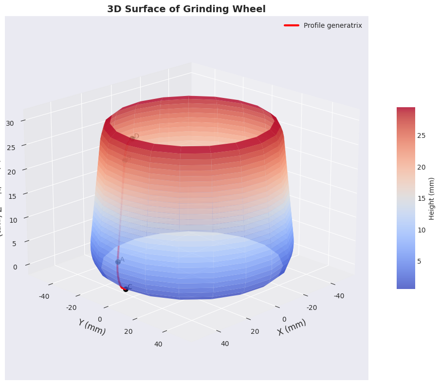
代码实现:参数化分析与半径函数可视化
python
import numpy as np
import matplotlib.pyplot as plt

# 重新定义GrindingWheelProfile类确保独立运行
class GrindingWheelProfile:
    def __init__(self, R=50.0, R_wl=5.0, R_wr=5.0, H=30.0, kappa=15.0):
        self.R = R
        self.R_wl = R_wl
        self.R_wr = R_wr
        self.H = H
        self.kappa = np.deg2rad(kappa)
        self._calculate_parameters()

    def _calculate_parameters(self):
        self.alpha_0 = np.pi/2 + self.kappa
        self.alpha_1 = np.pi/2 - self.kappa
        self.h_L = 2 * self.R_wl * (np.sin(self.alpha_0/2)**2)
        self.h_r = self.R_wr * np.tan(self.alpha_1/2)
        self.h_m = self.H - self.h_L - self.h_r
        self.R_hL = self.R - self.R_wl + np.sqrt(self.R_wl**2 - (self.R_wl - self.h_L)**2)

    def R_h(self, h):
        h = np.asarray(h)
        R = np.zeros_like(h)

        left_mask = h <= self.h_L
        middle_mask = (h > self.h_L) & (h <= self.H - self.h_r)
        right_mask = h > self.H - self.h_r

        if np.any(left_mask):
            h_left = h[left_mask]
            R[left_mask] = self.R - self.R_wl + np.sqrt(self.R_wl**2 - (self.R_wl - h_left)**2)

        if np.any(middle_mask):
            h_middle = h[middle_mask]
            R[middle_mask] = self.R_hL - (h_middle - self.h_L) * np.tan(self.kappa)

        if np.any(right_mask):
            h_right = h[right_mask]
            term = (self.R_wr - self.H + h_right)
            R[right_mask] = (self.R_hL - self.h_m * np.tan(self.kappa) -
                            self.R_wr * np.cos(self.kappa) +
                            np.sqrt(self.R_wr**2 - term**2))

        return R

# 创建砂轮对象
wheel = GrindingWheelProfile(R=50.0, R_wl=5.0, R_wr=5.0, H=30.0, kappa=15.0)

# 获取参数
h_L = wheel.h_L
h_r = wheel.h_r
alpha_0 = wheel.alpha_0
alpha_1 = wheel.alpha_1
R_wl = wheel.R_wl
R_wr = wheel.R_wr
R_hL = wheel.R_hL
h_m = wheel.h_m
kappa = wheel.kappa
H = wheel.H

# 创建多子图
fig, axes = plt.subplots(2, 2, figsize=(14, 10))
fig.suptitle('Parametric Analysis of Grinding Wheel', fontsize=16, fontweight='bold')

# 1. 半径函数分段图
ax1 = axes[0, 0]
h = np.linspace(0, H, 500)
R = wheel.R_h(h)
ax1.plot(h, R, 'b-', linewidth=2)
ax1.axvline(x=h_L, color='r', linestyle='--', alpha=0.5, label=f'h_L={h_L:.2f}')
ax1.axvline(x=H-h_r, color='g', linestyle='--', alpha=0.5, label=f'H-h_r={H-h_r:.2f}')
ax1.set_xlabel('h (mm)')
ax1.set_ylabel('R(h) (mm)')
ax1.set_title('Radius Function Segmentation')
ax1.grid(True, alpha=0.3)
ax1.legend()

# 2. 左侧圆弧参数化
ax2 = axes[0, 1]
alpha_AC = np.linspace(0, alpha_0, 100)
h_AC = 2 * R_wl * (np.sin(alpha_AC/2)**2)  # 公式(2-5)
R_AC = wheel.R - R_wl + np.sqrt(R_wl**2 - (R_wl - h_AC)**2)
ax2.plot(alpha_AC, h_AC, 'r-', label='h(α_AC)')
ax2.plot(alpha_AC, R_AC, 'b-', label='R(α_AC)')
ax2.set_xlabel('α_AC (rad)')
ax2.set_ylabel('Value (mm)')
ax2.set_title('Left Arc Parameterization')
ax2.legend()
ax2.grid(True, alpha=0.3)

# 3. 右侧圆弧参数化
ax3 = axes[1, 0]
alpha_BD = np.linspace(0, alpha_1, 100)
h_BD = H - 2 * R_wr * (np.sin(alpha_BD/2)**2)  # 公式(2-6)
term = R_wr - H + h_BD
R_BD = (R_hL - h_m * np.tan(kappa) - R_wr * np.cos(kappa) +
        np.sqrt(R_wr**2 - term**2))
ax3.plot(alpha_BD, h_BD, 'r-', label='h(α_BD)')
ax3.plot(alpha_BD, R_BD, 'b-', label='R(α_BD)')
ax3.set_xlabel('α_BD (rad)')
ax3.set_ylabel('Value (mm)')
ax3.set_title('Right Arc Parameterization')
ax3.legend()
ax3.grid(True, alpha=0.3)

# 4. 锥面段线性关系
ax4 = axes[1, 1]
h_mid = np.linspace(h_L, H-h_r, 100)
R_mid = R_hL - (h_mid - h_L) * np.tan(kappa)
ax4.plot(h_mid, R_mid, 'g-', linewidth=2)
ax4.set_xlabel('h (mm)')
ax4.set_ylabel('R(h) (mm)')
ax4.set_title(f'Conical Segment (κ={np.rad2deg(kappa):.1f}°)')
ax4.text(0.05, 0.95, f'Slope: -tan(κ) = {-np.tan(kappa):.3f}',
         transform=ax4.transAxes, verticalalignment='top')
ax4.grid(True, alpha=0.3)

plt.tight_layout()
plt.show()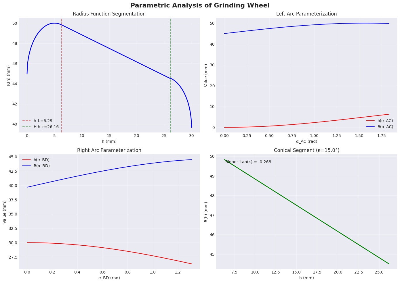
代码实现:不同锥角对比分析
python
import numpy as np
import matplotlib.pyplot as plt

# 定义GrindingWheelProfile类
class GrindingWheelProfile:
    def __init__(self, R=50.0, R_wl=5.0, R_wr=5.0, H=30.0, kappa=15.0):
        self.R = R
        self.R_wl = R_wl
        self.R_wr = R_wr
        self.H = H
        self.kappa = np.deg2rad(kappa)
        self._calculate_parameters()

    def _calculate_parameters(self):
        self.alpha_0 = np.pi/2 + self.kappa
        self.alpha_1 = np.pi/2 - self.kappa
        self.h_L = 2 * self.R_wl * (np.sin(self.alpha_0/2)**2)
        self.h_r = self.R_wr * np.tan(self.alpha_1/2)
        self.h_m = self.H - self.h_L - self.h_r
        self.R_hL = self.R - self.R_wl + np.sqrt(self.R_wl**2 - (self.R_wl - self.h_L)**2)

    def R_h(self, h):
        h = np.asarray(h)
        R = np.zeros_like(h)

        left_mask = h <= self.h_L
        middle_mask = (h > self.h_L) & (h <= self.H - self.h_r)
        right_mask = h > self.H - self.h_r

        if np.any(left_mask):
            h_left = h[left_mask]
            R[left_mask] = self.R - self.R_wl + np.sqrt(self.R_wl**2 - (self.R_wl - h_left)**2)

        if np.any(middle_mask):
            h_middle = h[middle_mask]
            R[middle_mask] = self.R_hL - (h_middle - self.h_L) * np.tan(self.kappa)

        if np.any(right_mask):
            h_right = h[right_mask]
            term = (self.R_wr - self.H + h_right)
            R[right_mask] = (self.R_hL - self.h_m * np.tan(self.kappa) -
                            self.R_wr * np.cos(self.kappa) +
                            np.sqrt(self.R_wr**2 - term**2))

        return R

# 创建不同锥角的砂轮对象
wheels = [
    GrindingWheelProfile(R=50, R_wl=5, R_wr=5, H=30, kappa=0),   # 无锥角
    GrindingWheelProfile(R=50, R_wl=5, R_wr=5, H=30, kappa=15),  # 中锥角
    GrindingWheelProfile(R=50, R_wl=5, R_wr=5, H=30, kappa=30)   # 大锥角
]

titles = ['No Taper (κ=0°)', 'Medium Taper (κ=15°)', 'Large Taper (κ=30°)']

# 创建对比图
fig, axes = plt.subplots(1, 3, figsize=(15, 5))
fig.suptitle('Comparison of Grinding Wheel Profiles with Different Taper Angles',
             fontsize=14, fontweight='bold')

for ax, wheel, title in zip(axes, wheels, titles):
    # 生成轮廓点
    h_points = np.linspace(0, wheel.H, 500)
    R_points = wheel.R_h(h_points)

    # 绘制轮廓线
    ax.plot(h_points, R_points, 'b-', linewidth=2)
    ax.plot(h_points, -R_points, 'b--', linewidth=1, alpha=0.5)

    # 绘制中心线
    ax.axhline(y=0, color='k', linestyle='-', linewidth=0.5, alpha=0.3)

    # 获取关键点
    h_L = wheel.h_L
    h_r = wheel.h_r
    R_hL = wheel.R_hL

    # 计算关键点
    C = (0, wheel.R - wheel.R_wl)
    A = (h_L, R_hL)
    h_B = wheel.H - h_r
    R_B = R_hL - (h_B - h_L) * np.tan(wheel.kappa)
    B = (h_B, R_B)
    D = (wheel.H, wheel.R_h(np.array([wheel.H]))[0])

    # 绘制关键点
    key_points = [C, A, B, D]
    point_names = ['C', 'A', 'B', 'D']
    colors = ['r', 'g', 'm', 'c']

    for (h, R), name, color in zip(key_points, point_names, colors):
        ax.plot(h, R, f'{color}o', markersize=6, markeredgecolor='k')
        ax.text(h, R+1, name, fontsize=9, ha='center')

    ax.set_title(title)
    ax.grid(True, alpha=0.3)
    ax.axis('equal')

    # 添加参数信息
    info_text = f"""
    h_L = {h_L:.2f} mm
    h_r = {h_r:.2f} mm
    h_m = {wheel.h_m:.2f} mm
    α₀ = {np.rad2deg(wheel.alpha_0):.1f}°
    α₁ = {np.rad2deg(wheel.alpha_1):.1f}°
    """
    ax.text(0.05, 0.95, info_text, transform=ax.transAxes, fontsize=8,
            verticalalignment='top', bbox=dict(boxstyle='round', facecolor='wheat', alpha=0.5))

# 设置公共标签
for ax in axes:
    ax.set_xlabel('Axial position h (mm)')
axes[0].set_ylabel('Radius R(h) (mm)')

plt.tight_layout()
plt.show()

# 打印对比数据
print("=" * 70)
print("Comparison of Parameters for Different Taper Angles")
print("=" * 70)
print(f"{'Taper Angle':<15} {'α₀ (°)':<10} {'α₁ (°)':<10} {'h_L (mm)':<12} {'h_r (mm)':<12} {'h_m (mm)':<12}")
print("-" * 70)

for wheel, title in zip(wheels, titles):
    print(f"{title:<15} {np.rad2deg(wheel.alpha_0):<10.1f} {np.rad2deg(wheel.alpha_1):<10.1f} "
          f"{wheel.h_L:<12.2f} {wheel.h_r:<12.2f} {wheel.h_m:<12.2f}")

print("=" * 70)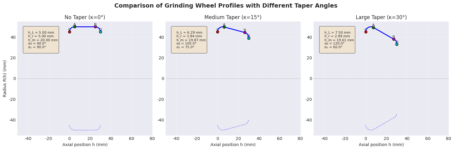
分析与讨论
数学模型的有效性验证
通过Python实现,我们验证了砂轮轮廓参数化模型的有效性。半径函数 R(h)R(h)R(h) 的分段定义能够精确描述包含圆弧过渡段和锥面段的复杂轮廓。关键特征点 CCC、AAA、BBB、DDD 的计算结果与几何预期一致。
参数敏感性分析
从不同锥角的对比分析可以看出:
- 锥角 κ\kappaκ 的影响 :随着 κ\kappaκ 增大,左侧最大中心角 α0\alpha_0α0 增大,右侧最大中心角 α1\alpha_1α1 减小,锥面段斜率绝对值增大。
- 圆弧段长度变化 :锥角增大导致左侧圆弧段长度 hLh_LhL 增加,右侧圆弧段长度 hrh_rhr 减小,锥面段长度 hmh_mhm 相应变化。
- 轮廓形状变化:无锥角时,砂轮轮廓近似为带圆角的圆柱;随着锥角增大,轮廓逐渐变为锥形。
计算精度与效率
通过自适应参数化方法,将圆弧段用中心角 α\alphaα 作为离散控制参数,可以提高包络计算的精度。半径函数的分段定义使得计算具有 O(1)O(1)O(1) 的时间复杂度,适合实时计算和仿真应用。
结论
本文建立了完整的砂轮轮廓参数化数学模型,并提供了Python实现。模型能够精确描述包含圆弧过渡段和锥面段的复杂砂轮轮廓,为精密磨削加工中的包络计算、刀具轨迹规划和加工仿真提供了理论基础和计算工具。