机器学习（9-2）

线性SVM分类

python 复制代码

import numpy as np
import matplotlib.pyplot as plt

from sklearn.datasets import make_blobs
x,y = make_blobs(
    n_samples=40,
    centers=2,
    random_state=0
)

from sklearn.svm import LinearSVC
## 软间隔公式所对应的C
clf = LinearSVC(C=1)
clf.fit(x,y)

# 决策边界
def decision_boundary_plot(x,y,clf):
    # 确定画图范围：向外扩 1 个单位，避免边界贴边
    axis_x1_min, axis_x1_max = x[:, 0].min() - 1, x[:, 0].max() + 1
    axis_x2_min, axis_x2_max = x[:, 1].min() - 1, x[:, 1].max() + 1
    # 构造二维网格点（关键）
    x1, x2 = np.meshgrid(
        np.arange(axis_x1_min, axis_x1_max, 0.01),
        np.arange(axis_x2_min, axis_x2_max, 0.01),
    )
    # 对每个网格点做预测，得到 整片平面的分类结果
    z = clf.predict(np.c_[x1.ravel(), x2.ravel()])
    # 预测结果变回网格形状，每个网格点都有一个类别
    z = z.reshape(x1.shape)

    from matplotlib.colors import ListedColormap
    # 自定义颜色
    custom_cmap = ListedColormap(['#F5B9EF','#FFFFFF','#F9F9CB'])
    # 画决策区域 / 决策边界，不同颜色交界处 = 决策边界
    plt.contourf(x1,x2,z,cmap=custom_cmap)
    plt.scatter(x[:,0],x[:,1],c=y)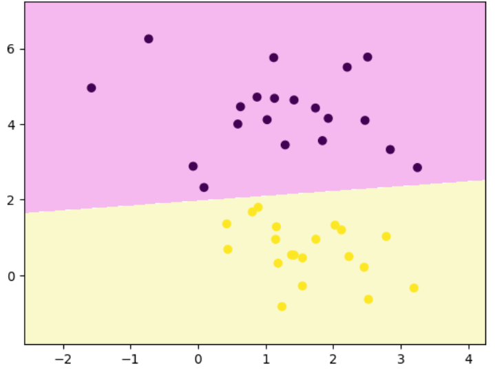

绘制margin

python 复制代码

## 绘制margin
def plot_svm_margin(x,y,clf,ax=None):
    from sklearn.inspection import DecisionBoundaryDisplay
    DecisionBoundaryDisplay.from_estimator(
        clf,
        x,
        ax = ax,
        grid_resolution=50,
        plot_method='contour',
        colors='k',
        levels=[-1,0,1],
        alpha=0.5,
        linestyles=['--','-','--']
    )
    plt.scatter(x[:,0],x[:,1],c=y)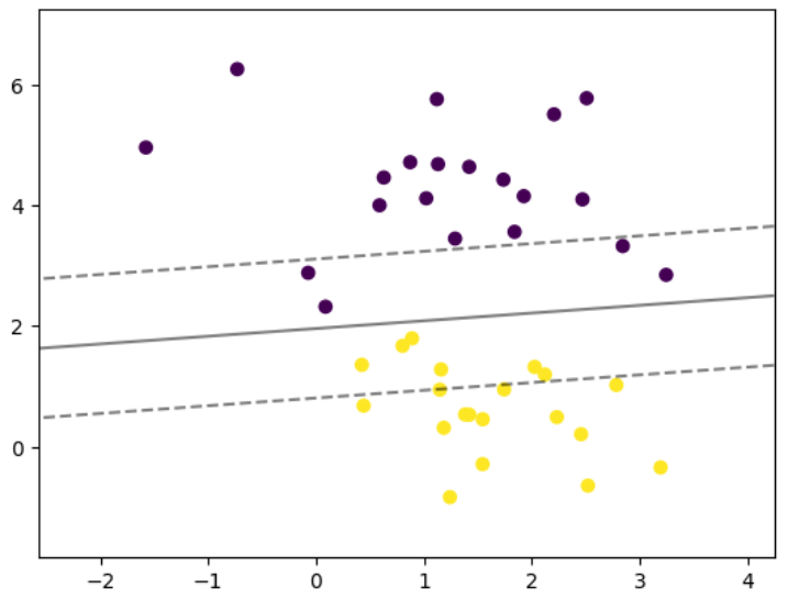

不同参数C值的margin图像

python 复制代码

## 绘制不同参数的图像
plt.rcParams["figure.figsize"] = (12,8)

params = [0.1,1,10,100]
for i,c in enumerate(params):
    clf = LinearSVC(C=c,random_state=0)
    clf.fit(x,y)
    ## 绘制两行两列的子图
    ax = plt.subplot(2,2,i+1)
    plt.title("C:{0}".format(c))
    plot_svm_margin(x,y,clf,ax)

plt.show()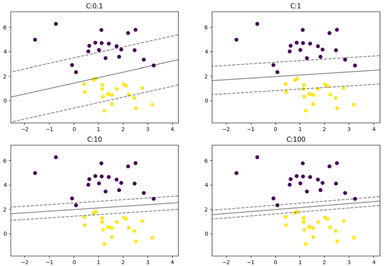

多分类问题

python 复制代码

from sklearn import datasets
iris = datasets.load_iris()

x = iris.data
y = iris.target

## OVR:多分类的方式，一对其他，LinearSVC不支持OVO，默认就是OVR
clf = LinearSVC(C=0.1,multi_class='ovr',random_state=0)
clf.fit(x,y)

非线性SVM分类

数据准备

python 复制代码

import numpy as np
import matplotlib.pyplot as plt
from sklearn.datasets import make_moons
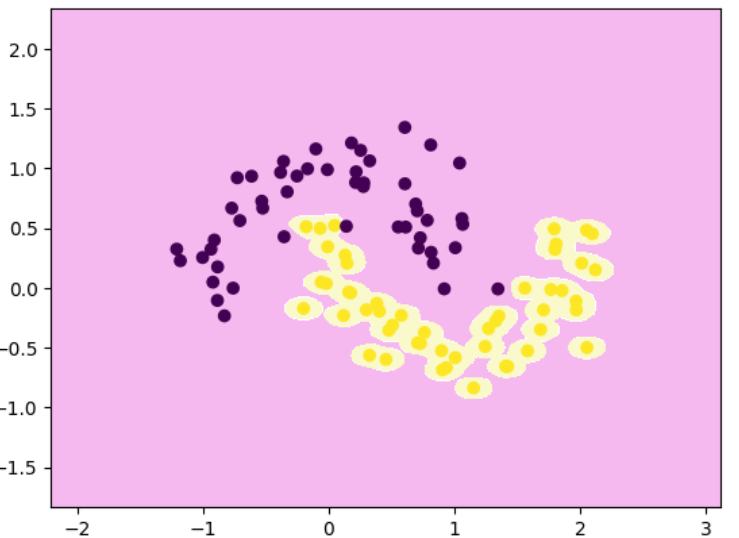
x,y = make_moons(n_samples=100,noise=0.2,random_state=0)

多项式特征解决非线性问题

python 复制代码

from sklearn.preprocessing import PolynomialFeatures,StandardScaler
from sklearn.pipeline import Pipeline

poly_svc = Pipeline([
    ("poly",PolynomialFeatures(degree=3)),
    ("std_scaler",StandardScaler()),
    ("linearSVC",LinearSVC())
])

poly_svc.fit(x,y)

decision_boundary_plot(x,y,poly_svc)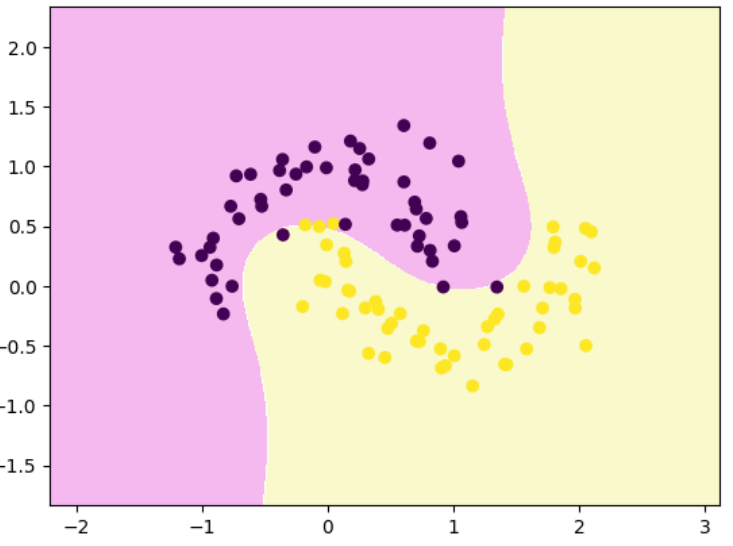

核函数解决非线性问题

python 复制代码

# 多项式核函数
from sklearn.svm import SVC
poly_svc = Pipeline([
    ("std_scaler",StandardScaler()),
    ("polySVC",SVC(kernel='poly',degree=3))
])
poly_svc.fit(x,y)

# 高斯核函数
# coef0 主要是在非线性核函数（特别是多项式核和RBF核）中控制模型对样本间距离或特征交互的"敏感度"
# 调整gamma:1,0.1,10,100
rbf_svc = Pipeline([
    ("std_scaler",StandardScaler()),
    ("polySVC",SVC(kernel='rbf',gamma=1))
])
rbf_svc.fit(x,y)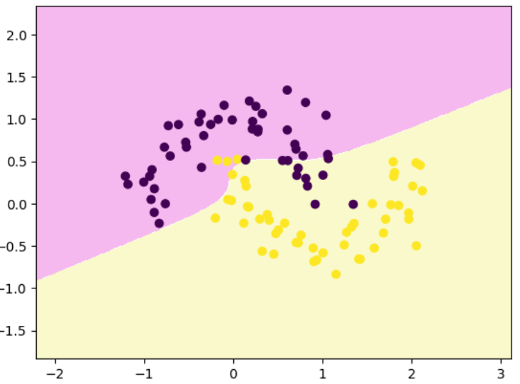

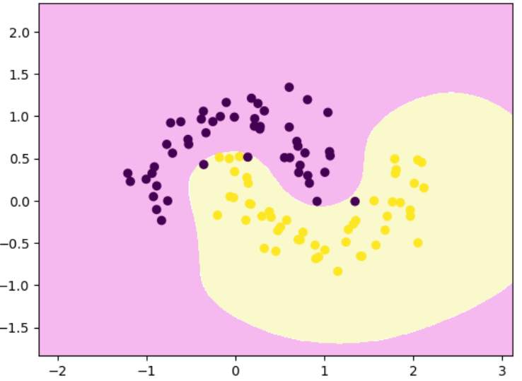
调整高斯函数的参数值

python 复制代码

# 调整gamma:100，发生过拟合
rbf_svc = Pipeline([
    ("std_scaler",StandardScaler()),
    ("polySVC",SVC(kernel='rbf',gamma=100))
])
rbf_svc.fit(x,y)
decision_boundary_plot(x,y,rbf_svc)