【LLM原理学习】N-gram 语言模型实战教学指南（从原理到代码)

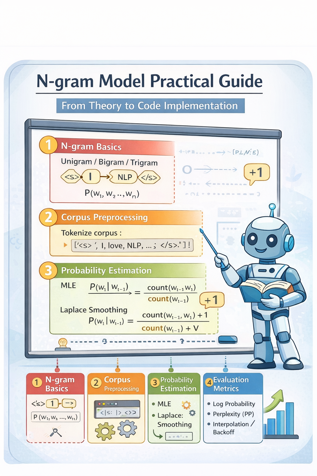
本文是一篇偏教学风格的 N-gram 实战技术博客，结合完整 Python 代码，逐步讲解：

• 什么是 N-gram
• 如何构建 Unigram / Bigram / Trigram
• 如何计算语言模型概率
• 什么是拉普拉斯平滑（Laplace Smoothing）
• 如何评估一句话的概率
  

第一章：N-gram 语言模型基础

1.1 什么是语言模型？

​ 在自然语言处理中，我们希望估计一句话出现的概率有多大 ：
P ( w 1 , w 2 , ... , w n ) P(w_1, w_2, \dots, w_n) P(w1,w2,...,wn)

​ 其中， w i w_i wi表示句子中的第 i i i个词。

• 语言模型的核心任务是：判断一句话在自然语言中出现的合理性。

  然而，真实语言存在复杂的长距离依赖关系，例如"The book that I bought yesterday is interesting.

• 因此，要精确建模这种依赖几乎不可行，因此需要对问题进行简化。

1.2 链式法则与概率分解

​ 根据概率的链式法则（Chain Rule）：
P ( w 1 , w 2 , ... , w n ) = ∏ i = 1 n P ( w i ∣ w 1 , ... , w i − 1 ) P(w_1, w_2, \dots, w_n) = \prod_{i=1}^{n} P(w_i \mid w_1, \dots, w_{i-1}) P(w1,w2,...,wn)=i=1∏nP(wi∣w1,...,wi−1)

​ 这个公式是语言模型的数学基础， 但该公式的条件概率依赖历史所有词，参数规模指数级增长，无法直接估计。

1.3 马尔可夫假设与 N-gram 模型

​ 为降低建模复杂度，引入 马尔可夫假设（Markov Assumption） ：当前词只依赖前 N − 1 N-1 N−1个词。

​ 于是得到 N-gram 语言模型：

• Unigram ：只考虑当前词
  P ( w i ) P(w_i) P(wi)

• Bigram ：只依赖前 1 个词
  P ( w i ∣ w i − 1 ) P(w_i \mid w_{i-1}) P(wi∣wi−1)

• Trigram ：只依赖前 2 个词
  P ( w i ∣ w i − 2 , w i − 1 ) P(w_i \mid w_{i-2}, w_{i-1}) P(wi∣wi−2,wi−1)

  N-gram 模型的核心思想是：用局部上下文近似全局语言依赖关系。

1.4 N-gram 模型的直观理解

​ 以 Bigram 为例，句子概率可以近似为：
P ( w 1 , ... , w n ) ≈ ∏ i = 2 n P ( w i ∣ w i − 1 ) P(w_1, \dots, w_n) \approx \prod_{i=2}^{n} P(w_i \mid w_{i-1}) P(w1,...,wn)≈i=2∏nP(wi∣wi−1)

​ 即一句话的概率 = 相邻词对概率的连乘。

​ 例如，对于<s> I love language models </s>

​ 对应 Bigram：

(<s>, I)
(I, love)
(love, language)
(language, models)
(models, </s>)

​ 模型通过统计这些词对的频率来学习语言规律。

第二章：语料预处理与分词

2.1 分词与句子边界标记

​ 语言模型必须知道句子的起始与终止位置，因此需要加入边界标记：

from nltk.tokenize import word_tokenize

def tokenize_with_boundaries(sentence):
    tokens = word_tokenize(sentence)
    return ["<s>"] + tokens + ["</s>"]

​ 其中，<s> 表示句子开始，</s> 表示句子结束

​ 这样模型可以学习：
P ( w 1 ∣ < s > ) , P ( < / s > ∣ w n ) P(w_1 \mid <s>), P(</s> \mid w_n) P(w1∣<s>),P(</s>∣wn)

2.2 构建语料分词结果

def tokenize_corpus(corpus):
    tokenized_corpus = [tokenize_with_boundaries(s) for s in corpus]
    return tokenized_corpus

​ 例如：

I love natural language processing.

​ 被转换为：

<s> I love natural language processing . </s>

第三章：N-gram 统计建模

​ 本章介绍如何从语料中构建 Unigram、Bigram 和 Trigram 的频次统计，这是语言模型概率估计的基础。

3.1 Unigram 统计

from collections import Counter

def build_unigram(tokenized_corpus):
    unigram_counts = Counter()
    for tokens in tokenized_corpus:
        unigram_counts.update(tokens)
    return unigram_counts

(1) 数学定义

• Unigram 的统计量定义为： count ( w ) \text{count}(w) count(w)

​ 表示词 w w w在整个语料中的出现次数。

• 对应的概率估计为：
  P ( w ) = c o u n t ( w ) ∑ w ′ c o u n t ( w ′ ) P(w) = \frac{count(w)}{\sum_{w'} count(w')} P(w)=∑w′count(w′)count(w)
  即词的经验频率估计（Maximum Likelihood Estimation, MLE）。

(2) 理论说明

​ Unigram 模型假设每个词是独立生成的，与上下文无关。

​ 因此句子概率为：
P ( w 1 , ... , w n ) = ∏ i = 1 n P ( w i ) P(w_1, \dots, w_n) = \prod_{i=1}^{n} P(w_i) P(w1,...,wn)=i=1∏nP(wi)

​ 该假设显然过于简单，但 Unigram 是所有语言模型的基础统计单元。

3.2 Bigram 统计

from collections import Counter

def build_bigram(tokenized_corpus):
    bigram_counts = Counter()
    for tokens in tokenized_corpus:
        bigram_counts.update(ngrams(tokens, 2))
    return bigram_counts

​ 例如，对于句子<s> I love language models </s>

​ Bigram 序列为：

(<s>, I)
(I, love)
(love, language)
(language, models)
(models, </s>)

(1) 数学定义

​ Bigram 定义为连续两个词的组合：
( w i − 1 , w i ) (w_{i-1}, w_i) (wi−1,wi)

​ 统计量为：
count ( w i − 1 , w i ) \text{count}(w_{i−1}, w_{i}) count(wi−1,wi)

​ 条件概率估计公式为：
P ( w i ∣ w i − 1 ) = count ( w i − 1 , w i ) count ( w i − 1 ) P(w_i \mid w_{i−1})= \frac{\text{count}(w_{i-1}, w_i)}{\text{count}(w_{i−1})} P(wi∣wi−1)=count(wi−1)count(wi−1,wi)

(2) 理论说明

​ Bigram 模型假设当前词只依赖前一个词。

​ 因此句子概率近似为：
P ( w 1 , ... , w n ) ≈ ∏ i = 2 n P ( w i ∣ w i − 1 ) P(w_1, \dots, w_n) \approx \prod_{i=2}^{n} P(w_i \mid w_{i-1}) P(w1,...,wn)≈i=2∏nP(wi∣wi−1)

​ 这比 Unigram 模型捕捉了局部上下文信息。

3.3 Trigram 统计

from collections import Counter

def build_trigram(tokenized_corpus):
    trigram_counts = Counter()
    for tokens in tokenized_corpus:
        trigram_counts.update(ngrams(tokens, 3))
    return trigram_counts

(1) 数学定义

​ Trigram 定义为连续三个词的组合：
( w i − 2 , w i − 1 , w i ) (w_{i-2}, w_{i-1}, w_i) (wi−2,wi−1,wi)

​ 条件概率估计为：
P ( w i ∣ w i − 2 , w i − 1 ) = count ( w i − 2 , w i − 1 , w i ) count ( w i − 2 , w i − 1 ) P(w_i \mid w_{i-2}, w_{i-1}) = \frac{\text{count}(w_{i-2}, w_{i-1}, w_i)}{\text{count}(w_{i-2}, w_{i-1})} P(wi∣wi−2,wi−1)=count(wi−2,wi−1)count(wi−2,wi−1,wi)

(2) 理论说明

​ Trigram 模型假设当前词依赖前两个词。

​ 例如对于("New", "York", "City")，Trigram 能区分New York City和New York Times，这种能力是 Bigram 无法完全捕捉的。

3.4 小结

• Unigram 统计词频，用于估计词的先验概率
• Bigram/Trigram 建模上下文条件概率
• N N N越大，语言模型表达能力越强，但稀疏性与参数规模爆炸，这直接导致必须引入 平滑技术（Smoothing）

第四章：稀疏性问题与拉普拉斯平滑

4.1 数据稀疏问题

Zero Probability Problem

​ 随着 N N N增大，参数空间呈指数级增长。

• 设词表大小为 V V V，则：

模型	参数规模
Unigram	O ( V ) O(V) O(V)
Bigram	O ( V 2 ) O(V^2) O(V2)
Trigram	O ( V 3 ) O(V^3) O(V3)

​ 例如，若 V = 50 , 000 V = 50,000 V=50,000，Bigram 参数量 ≈ 2.5 × 10 9 2.5 \times 10^{9} 2.5×109，Trigram 参数量 ≈ 1.25 × 10 14 1.25 \times 10^{14} 1.25×1014

​ 几乎所有 n-gram 在语料中不会出现，导致概率为 0 ，这就是 数据稀疏性问题（Data Sparsity）。

4.2 拉普拉斯平滑（Laplace Smoothing）

​ 为解决零概率问题，引入加一平滑（Add-One Smoothing）。

(1) 理论说明

​ 拉普拉斯平滑的数学公式：
P ( w i ∣ w i − 1 ) = c o u n t ( w i − 1 , w i ) + 1 c o u n t ( w i − 1 ) + V P(w_i \mid w_{i-1}) = \frac{count(w_{i-1}, w_i) + 1}{count(w_{i-1}) + V} P(wi∣wi−1)=count(wi−1)+Vcount(wi−1,wi)+1

​ 其中， V V V是词表大小（Vocabulary Size）

​ 拉普拉斯平滑假设每个可能的词组合至少出现过一次（虚拟观测）。

​ 因此，未出现的 n-gram 不再概率为 0。所有概率重新归一化

(2) 拉普拉斯平滑代码实现

def bigram_laplace_prob(w1, w2, bigram_counts, unigram_counts, V):
    """
    P(w2 | w1) = (count(w1,w2) + 1) / (count(w1) + V)
    """
    count_w1 = unigram_counts.get(w1, 0)
    count_bigram = bigram_counts.get((w1, w2), 0)
    return (count_bigram + 1) / (count_w1 + V)

• 代码对应数学公式

  代码变量	数学符号	含义
  count_bigram	(count(w_{i-1}, w_i))	bigram 频次
  count_w1	(count(w_{i-1}))	上下文频次
  V	(V)	词表大小

(3) Laplace 平滑的统计学解释

​ 从贝叶斯角度，拉普拉斯平滑等价于对多项式分布使用 Dirichlet(1) 先验：
P ( θ ) ∼ D i r i c h l e t ( 1 , 1 , ... , 1 ) P(\theta) \sim Dirichlet(1,1,\dots,1) P(θ)∼Dirichlet(1,1,...,1)

​ 即假设每个词组合先验出现 1 次。

4.3 句子概率的平滑估计

​ 在 Bigram 模型下：
P ( w 1 , ... , w n ) = ∏ i = 2 n P ( w i ∣ w i − 1 ) P(w_1, \dots, w_n) = \prod_{i=2}^{n} P(w_i \mid w_{i-1}) P(w1,...,wn)=i=2∏nP(wi∣wi−1)

​ 加入 Laplace 平滑：
P ( w 1 , ... , w n ) = ∏ i = 2 n c o u n t ( w i − 1 , w i ) + 1 c o u n t ( w i − 1 ) + V P(w_1, \dots, w_n) = \prod_{i=2}^{n} \frac{count(w_{i-1}, w_i) + 1}{count(w_{i-1}) + V} P(w1,...,wn)=i=2∏ncount(wi−1)+Vcount(wi−1,wi)+1

(1) 对应代码实现

def sentence_bigram_laplace_prob(tokens, bigram_counts, unigram_counts):
    V = len(unigram_counts)
    total_prob = 1.0

    for w1, w2 in ngrams(tokens, 2):
        p = bigram_laplace_prob(w1, w2, bigram_counts, unigram_counts, V)
        total_prob *= p

    return total_prob

4.4 拉普拉斯平滑缺点

​ 尽管 Laplace 平滑简单，但存在严重问题：

• 对高频事件影响较大

• 对大词表严重过度平滑

• 概率分布被过度均匀化

  因此在真实语言模型中几乎不使用。

第五章：语言模型评估与工程实践

本章介绍如何评估 N-gram 模型性能，并给出工程实践中常用指标与改进方法。

5.1 句子对数概率（Log Probability）

​ 在实际计算中，句子概率是多个条件概率的乘积：
P ( w 1 , ... , w n ) = ∏ i = 2 n P ( w i ∣ w i − 1 ) P(w_1, \dots, w_n) = \prod_{i=2}^{n} P(w_i \mid w_{i-1}) P(w1,...,wn)=i=2∏nP(wi∣wi−1)

​ 但每个概率通常远小于 1，直接连乘会导致 数值下溢（Underflow）。

​ 因此实际工程中使用对数概率：
log ⁡ P ( w 1 , ... , w n ) = ∑ i = 2 n log ⁡ P ( w i ∣ w i − 1 ) \log P(w_1, \dots, w_n) = \sum_{i=2}^{n} \log P(w_i \mid w_{i-1}) logP(w1,...,wn)=i=2∑nlogP(wi∣wi−1)

• Python 实现

import math

def sentence_log_prob(tokens, bigram_counts, unigram_counts):
    V = len(unigram_counts)
    log_prob = 0.0

    for w1, w2 in ngrams(tokens, 2):
        p = bigram_laplace_prob(w1, w2, bigram_counts, unigram_counts, V)
        log_prob += math.log(p)

    return log_prob

5.2 困惑度（Perplexity）

​ 困惑度是语言模型的标准评价指标，用于衡量模型对测试语料的不确定性。

• 定义：
  PP ( W ) = exp ⁡ ( − 1 N ∑ i = 1 N log ⁡ P ( w i ∣ w i − 1 ) ) \text{PP}(W) = \exp\left(-\frac{1}{N} \sum_{i=1}^{N} \log P(w_i \mid w_{i-1})\right) PP(W)=exp(−N1i=1∑NlogP(wi∣wi−1))

• 直观理解：模型在预测下一个词时平均有多少种"困惑选择"

(1) Python 实现

def perplexity(tokens, bigram_counts, unigram_counts):
    N = len(tokens) - 1
    log_prob = sentence_log_prob(tokens, bigram_counts, unigram_counts)
    return math.exp(-log_prob / N)

​ 可以看到，这里计算时分母实际为 N − 1 N-1 N−1

​ 设句子：

<s> w_1 w_2 ... w_T </s>

​ 如果 tokens 长度是：
∣ W ∣ = T + 2 |W| = T + 2 ∣W∣=T+2

​ 那么Bigram的数量是：
∣ Bigrams ∣ = ∣ W ∣ − 1 |\text{Bigrams}| = |W| - 1 ∣Bigrams∣=∣W∣−1

​ 因为：
P ( w 1 , ⋯   , w T ) = ∏ t = 2 T P ( w i ∣ w i − 1 ) P(w_1, \cdots, w_T)=\prod_{t=2}^T P(w_i \mid w_{i−1}) P(w1,⋯,wT)=t=2∏TP(wi∣wi−1)

​ 因此条件概率个数为tokens-1。

(2) Perplexity 解释

• PP 越小 → 模型越好
• PP = 1 → 完美预测
• PP ≈ V → 接近随机猜词

5.3 N-gram 模型的局限性

​ 尽管 N-gram 是语言模型的基础，但存在根本缺陷：

(1) 长距离依赖问题

• N 只能捕捉有限上下文
• 无法建模句法与语义结构

(2) 参数爆炸

​ 参数规模： O ( V N ) O(V^N) O(VN)

​ 真实语言任务几乎不可存储。

(3) 数据稀疏问题

• 大多数 n-gram 永远不会出现
• 平滑方法只能缓解，不能根治