谐波检测之瞬时无功功率理论 ip-iq 检测法：从原理到实践

谐波检测瞬时无功功率理论ipiq检测法

在电力系统的复杂世界里，谐波问题一直是让人头疼的存在。谐波不仅会降低电能质量，还可能对各种电气设备造成损害。而瞬时无功功率理论中的 ip - iq 检测法，就如同一位可靠的侦探，能够精准地找出电力系统中的谐波成分。今天咱们就来好好唠唠这神奇的 ip - iq 检测法。

一、瞬时无功功率理论基础

瞬时无功功率理论是由日本学者赤木泰文等人提出的，它基于三相电路的瞬时功率分析，打破了传统功率理论在正弦稳态下的限制，适用于任意波形和不平衡的三相电路。

三相电路瞬时功率

对于三相三线制系统，设三相电压瞬时值为 \(ua\)、\(u b\)、\(uc\)，三相电流瞬时值为 \(i a\)、\(ib\)、\(ic\)。瞬时有功功率 \(p\) 和瞬时无功功率 \(q\) 定义如下：

\[

\begin{cases}

p = ua i a + ub i b + uc ic \\

q = \frac{1}{\sqrt{3}}[(ua - u b)ic + (u b - uc)i a + (uc - ua)i_b]

\end{cases}

\]

二、ip - iq 检测法原理

ip - iq 检测法的核心思想是将三相电流通过坐标变换，分解到相互垂直的两个轴上（通常称为 \(\alpha - \beta\) 坐标系），然后在这个坐标系下分离出基波有功电流和其他成分（谐波和无功电流）。

1. 坐标变换

首先进行 Clark 变换，将三相静止坐标系（abc 坐标系）变换到两相静止坐标系（\(\alpha - \beta\) 坐标系）。变换矩阵 \(C_{32}\) 为：

\[

C_{32} = \sqrt{\frac{2}{3}}

\begin{pmatrix}

1 & -\frac{1}{2} & -\frac{1}{2} \\

0 & \frac{\sqrt{3}}{2} & -\frac{\sqrt{3}}{2}

\end{pmatrix}

\]

三相电流 \(\mathbf{i}{abc} = \begin{pmatrix} i a \\ ib \\ ic \end{pmatrix}\) 经过 Clark 变换后得到 \(\alpha - \beta\) 坐标系下的电流 \(\mathbf{i}_{\alpha\beta}\)：

\[

\mathbf{i}{\alpha\beta} = C{32} \mathbf{i}_{abc}

\]

\[

\begin{pmatrix} i*{\alpha} \\ i*{\beta} \end{pmatrix} = \sqrt{\frac{2}{3}}

\begin{pmatrix}

1 & -\frac{1}{2} & -\frac{1}{2} \\

0 & \frac{\sqrt{3}}{2} & -\frac{\sqrt{3}}{2}

谐波检测瞬时无功功率理论ipiq检测法

\end{pmatrix}

\begin{pmatrix} ia \\ ib \\ i_c \end{pmatrix}

\]

接着进行 Park 变换，将 \(\alpha - \beta\) 坐标系变换到同步旋转坐标系（\(d - q\) 坐标系）。变换矩阵 \(C_{pq}\) 为：

\[

C_{pq} =

\begin{pmatrix}

\cos\theta & \sin\theta \\

-\sin\theta & \cos\theta

\end{pmatrix}

\]

其中 \(\theta\) 是同步旋转角，一般由锁相环（PLL）获取。\(\alpha - \beta\) 坐标系下的电流 \(\mathbf{i}{\alpha\beta}\) 经过 Park 变换后得到 \(d - q\) 坐标系下的电流 \(\mathbf{i}{dq}\)：

\[

\mathbf{i}{dq} = C{pq} \mathbf{i}_{\alpha\beta}

\]

\[

\begin{pmatrix} id \\ iq \end{pmatrix} =

\begin{pmatrix}

\cos\theta & \sin\theta \\

-\sin\theta & \cos\theta

\end{pmatrix}

\begin{pmatrix} i*{\alpha} \\ i*{\beta} \end{pmatrix}

\]

2. 电流分离

在 \(d - q\) 坐标系下，基波有功电流只存在于 \(d\) 轴（假设电压无畸变且三相平衡）。我们可以通过低通滤波器（LPF）提取出 \(d\) 轴电流中的直流分量 \(i_{d0}\)，它代表基波有功电流在 \(d\) 轴的分量。

然后通过逆变换，将提取到的基波有功电流分量变换回三相坐标系，从而得到三相基波有功电流。而原三相电流与基波有功电流的差值，就是谐波和无功电流。

三、代码实现与分析

下面以 Python 为例，简单实现一下 ip - iq 检测法的核心部分（这里为了简化，假设已经获取到三相电压和电流数据，并且省略了锁相环部分的实现）。

import numpy as np
import matplotlib.pyplot as plt
from scipy.signal import butter, lfilter


# 定义 Clark 变换矩阵
def clark_transform():
    return np.sqrt(2 / 3) * np.array([[1, -1 / 2, -1 / 2],
                                       [0, np.sqrt(3) / 2, -np.sqrt(3) / 2]])


# 定义 Park 变换矩阵
def park_transform(theta):
    return np.array([[np.cos(theta), np.sin(theta)],
                     [-np.sin(theta), np.cos(theta)]])


# 设计低通滤波器
def butter_lowpass(cutoff, fs, order=5):
    nyq = 0.5 * fs
    normal_cutoff = cutoff / nyq
    b, a = butter(order, normal_cutoff, btype='low', analog=False)
    return b, a


def butter_lowpass_filter(data, cutoff, fs, order=5):
    b, a = butter_lowpass(cutoff, fs, order=order)
    y = lfilter(b, a, data)
    return y


# 假设已经获取到三相电流数据（这里简单模拟）
time = np.linspace(0, 1, 1000)
fs = 1000  # 采样频率
i_a = np.sin(2 * np.pi * 50 * time) + 0.5 * np.sin(2 * np.pi * 150 * time)
i_b = np.sin(2 * np.pi * 50 * (time - 1 / 300)) + 0.5 * np.sin(2 * np.pi * 150 * (time - 1 / 300))
i_c = np.sin(2 * np.pi * 50 * (time - 2 / 300)) + 0.5 * np.sin(2 * np.pi * 150 * (time - 2 / 300))
i_abc = np.vstack((i_a, i_b, i_c))

# Clark 变换
C32 = clark_transform()
i_alpha_beta = C32.dot(i_abc)

# 假设已经获取到同步旋转角（这里简单模拟）
theta = 2 * np.pi * 50 * time
Cpq = park_transform(theta)
i_dq = np.array([Cpq.dot(i_alpha_beta[:, i]) for i in range(len(time))]).T

# 通过低通滤波器提取基波有功电流在 d 轴的分量
cutoff = 10  # 低通滤波器截止频率
i_d0 = butter_lowpass_filter(i_dq[0, :], cutoff, fs)

# 逆 Park 变换
i_alpha_beta_est = np.array([np.linalg.inv(Cpq[:, :, i]).dot(np.array([i_d0[i], 0])) for i in range(len(time))]).T

# 逆 Clark 变换
C23 = np.vstack((np.hstack((1, 0)), np.hstack((-1 / 2, np.sqrt(3) / 2)), np.hstack((-1 / 2, -np.sqrt(3) / 2))))
i_abc_est = C23.dot(i_alpha_beta_est)

# 谐波和无功电流
i_harmonic_reactive = i_abc - i_abc_est

# 绘图
plt.figure(figsize=(12, 8))
plt.subplot(3, 1, 1)
plt.plot(time, i_a, label='Original i_a')
plt.plot(time, i_abc_est[0, :], label='Estimated fundamental i_a')
plt.legend()
plt.title('Phase A Current')

plt.subplot(3, 1, 2)
plt.plot(time, i_b, label='Original i_b')
plt.plot(time, i_abc_est[1, :], label='Estimated fundamental i_b')
plt.legend()
plt.title('Phase B Current')

plt.subplot(3, 1, 3)
plt.plot(time, i_c, label='Original i_c')
plt.plot(time, i_abc_est[2, :], label='Estimated fundamental i_c')
plt.legend()
plt.title('Phase C Current')

plt.tight_layout()
plt.show()

代码分析

1. 变换矩阵定义 ：clarktransform**函数定义了 Clark 变换矩阵，park transform 函数根据给定的同步旋转角 \(\theta\) 生成 Park 变换矩阵。
2. 低通滤波器设计 ：butterlowpass**和 butter lowpass_filter 函数使用 Butterworth 滤波器设计并实现了低通滤波器，用于提取基波有功电流在 \(d\) 轴的直流分量。
3. 电流变换与提取：通过矩阵乘法依次进行 Clark 变换、Park 变换，将三相电流转换到 \(d - q\) 坐标系。然后利用低通滤波器提取 \(d\) 轴的基波有功电流分量 \(i_{d0}\)。接着通过逆 Park 变换和逆 Clark 变换将基波有功电流分量转换回三相坐标系，得到三相基波有功电流估计值。最后通过原三相电流减去估计的基波有功电流得到谐波和无功电流。
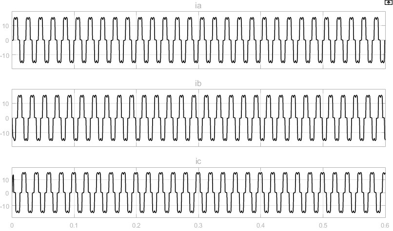
4. 绘图展示 ：使用 matplotlib 库绘制了三相原始电流和估计的基波有功电流，以便直观地观察谐波检测效果。

四、总结

瞬时无功功率理论的 ip - iq 检测法为电力系统中的谐波检测提供了一种有效的手段。通过巧妙的坐标变换和电流分离，能够准确地提取出基波有功电流，进而得到谐波和无功电流。虽然代码实现中做了一些简化，但基本原理都得以体现。在实际应用中，还需要考虑更多的因素，比如锁相环的精确实现、抗干扰措施等。希望通过这篇文章，大家对 ip - iq 检测法有了更深入的理解，能在电力相关的项目中更好地应用它。