机器学习-LASSO算法指南

一、LASSO是什么？

1.1 基本概念

LASSO（Least Absolute Shrinkage and Selection Operator，最小绝对收缩和选择算子）是一种用于线性回归的正则化方法。它的核心特点是既能防止过拟合，又能自动进行特征选择。

1.2 直观比喻

想象你要搬家：

普通线性回归：把所有东西都搬走，不管有没有用
Ridge回归（L2正则化）：把所有东西都带上，但每个都少带一点
LASSO回归（L1正则化）：只带最重要的几样东西，其他的直接扔掉

二、LASSO的数学原理

2.1 目标函数

LASSO在普通线性回归的基础上增加了一个L1惩罚项：

普通线性回归：最小化 Σ(yi−y^i)2Σ(y_i - ŷ_i)²Σ(yi−y^i)2
LASSO回归：最小化 [Σ(yi−y^i)2+λ∗Σ∣βj∣][Σ(y_i - ŷ_i)² + λ * Σ|β_j|][Σ(yi−y^i)2+λ∗Σ∣βj∣]

其中：

yiy_iyi 是实际值
y^i=β0+β1x1+β2x2+...+βpxpŷ_i = β₀ + β₁x₁ + β₂x₂ + ... + βₚxₚy^i=β0+β1x1+β2x2+...+βpxp 是预测值
λ（lambda）λ（lambda）λ（lambda）是正则化强度参数
∣βj∣|β_j|∣βj∣ 是系数βββ的绝对值

2.2 系数路径可视化

python 复制代码

import numpy as np
import matplotlib.pyplot as plt
from sklearn.linear_model import Lasso, LassoCV
from sklearn.preprocessing import StandardScaler

plt.rcParams['font.sans-serif'] = ['Heiti TC']
plt.rcParams['axes.unicode_minus'] = False

# 设置随机种子
np.random.seed(42)

# 创建模拟数据
n_samples = 100
n_features = 10

# 真实系数：只有前3个特征有影响，其他为0
true_coef = np.array([2.5, -1.8, 1.2, 0, 0, 0, 0, 0, 0, 0])

# 生成特征数据
X = np.random.randn(n_samples, n_features)

# 添加一点相关性
X[:, 3] = 0.6 * X[:, 0] + 0.4 * X[:, 1] + 0.1 * np.random.randn(n_samples)
X[:, 4] = 0.5 * X[:, 1] + 0.5 * np.random.randn(n_samples)

# 生成目标变量（加上噪声）
y = X @ true_coef + np.random.randn(n_samples) * 0.5

# 标准化数据（对LASSO很重要）
scaler = StandardScaler()
X_scaled = scaler.fit_transform(X)

# 创建不同的lambda值
lambdas = np.logspace(-4, 2, 100)  # 从10^-4到10^2

# 存储每个lambda下的系数
coefs = []

for lambd in lambdas:
    lasso = Lasso(alpha=lambd, max_iter=10000)
    lasso.fit(X_scaled, y)
    coefs.append(lasso.coef_)

coefs = np.array(coefs)

# 绘制系数路径图
plt.figure(figsize=(12, 8))

# 绘制每条系数路径
for i in range(n_features):
    plt.plot(lambdas, coefs[:, i], label=f'特征{i+1}', linewidth=2)

# 设置图形属性
plt.xscale('log')
plt.xlabel('正则化强度 λ (对数尺度)', fontsize=12)
plt.ylabel('系数值', fontsize=12)
plt.title('LASSO系数路径图', fontsize=16, fontweight='bold')
plt.grid(True, alpha=0.3)

# 添加垂直线标记最优lambda
lasso_cv = LassoCV(alphas=lambdas, cv=5, max_iter=10000, random_state=42)
lasso_cv.fit(X_scaled, y)
best_lambda = lasso_cv.alpha_
plt.axvline(x=best_lambda, color='red', linestyle='--', linewidth=2, 
           label=f'最优 λ = {best_lambda:.4f}')

# 高亮真实非零系数
for i in range(3):  # 前3个是真实特征
    plt.plot(lambdas, coefs[:, i], linewidth=3, alpha=0.8)

plt.legend(loc='upper right', fontsize=10, ncol=2)
plt.tight_layout()
plt.savefig('1.png',dpi=300, bbox_inches='tight')
plt.show()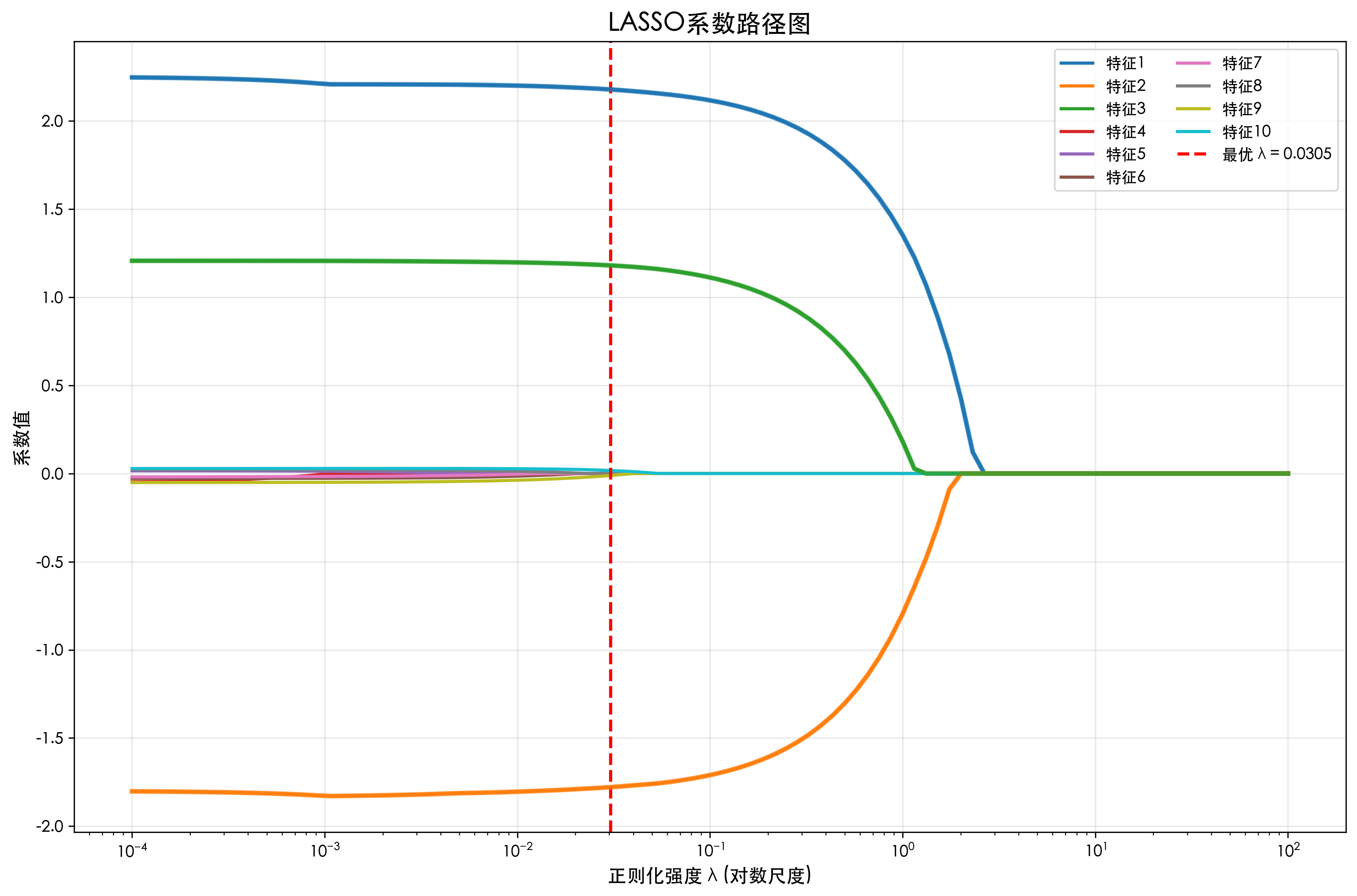

3.2 LASSO vs Ridge对比

python 复制代码

# LASSO和Ridge的对比
from sklearn.linear_model import Ridge
from mpl_toolkits.mplot3d import Axes3D

# 创建二维示例，便于可视化
np.random.seed(42)
X_2d = np.random.randn(50, 2)
true_coef_2d = np.array([1.5, 0.8])
y_2d = X_2d @ true_coef_2d + np.random.randn(50) * 0.3

# 标准化
scaler_2d = StandardScaler()
X_2d_scaled = scaler_2d.fit_transform(X_2d)

# 创建网格用于绘制等值线
beta1_range = np.linspace(-2, 3, 100)
beta2_range = np.linspace(-2, 3, 100)
B1, B2 = np.meshgrid(beta1_range, beta2_range)

# 计算损失函数
Z_ls = np.zeros_like(B1)  # 最小二乘损失
Z_l1 = np.zeros_like(B1)  # L1惩罚项
Z_l2 = np.zeros_like(B1)  # L2惩罚项

for i in range(len(beta1_range)):
    for j in range(len(beta2_range)):
        beta = np.array([B1[i, j], B2[i, j]])
        # 最小二乘损失
        Z_ls[i, j] = np.sum((y_2d - X_2d_scaled @ beta) ** 2)
        # L1惩罚
        Z_l1[i, j] = np.sum(np.abs(beta))
        # L2惩罚
        Z_l2[i, j] = np.sum(beta ** 2)

# LASSO目标函数
Z_lasso = Z_ls + 0.5 * Z_l1
# Ridge目标函数
Z_ridge = Z_ls + 0.5 * Z_l2

# 寻找最优解
lasso_2d = Lasso(alpha=0.5, max_iter=10000)
lasso_2d.fit(X_2d_scaled, y_2d)
lasso_coef = lasso_2d.coef_

ridge_2d = Ridge(alpha=0.5)
ridge_2d.fit(X_2d_scaled, y_2d)
ridge_coef = ridge_2d.coef_

# 绘制对比图
fig, axes = plt.subplots(1, 3, figsize=(18, 6))

# 1. LASSO约束区域（菱形）
axes[0].contour(B1, B2, Z_ls, levels=20, alpha=0.5, cmap='viridis')
axes[0].contour(B1, B2, Z_l1, levels=[0.5, 1, 1.5, 2], colors='red', linewidths=2)
axes[0].scatter(lasso_coef[0], lasso_coef[1], color='red', s=100, 
               marker='*', label='LASSO解')
axes[0].scatter(true_coef_2d[0], true_coef_2d[1], color='green', s=100,
               marker='o', label='真实系数')
axes[0].set_xlabel('β₁')
axes[0].set_ylabel('β₂')
axes[0].set_title('LASSO: L1约束（菱形）', fontsize=14)
axes[0].legend()
axes[0].grid(True, alpha=0.3)

# 2. Ridge约束区域（圆形）
axes[1].contour(B1, B2, Z_ls, levels=20, alpha=0.5, cmap='viridis')
axes[1].contour(B1, B2, Z_l2, levels=[0.5, 1, 2, 3], colors='blue', linewidths=2)
axes[1].scatter(ridge_coef[0], ridge_coef[1], color='blue', s=100,
               marker='*', label='Ridge解')
axes[1].scatter(true_coef_2d[0], true_coef_2d[1], color='green', s=100,
               marker='o', label='真实系数')
axes[1].set_xlabel('β₁')
axes[1].set_ylabel('β₂')
axes[1].set_title('Ridge: L2约束（圆形）', fontsize=14)
axes[1].legend()
axes[1].grid(True, alpha=0.3)

# 3. 三维可视化
ax = fig.add_subplot(133, projection='3d')
surf = ax.plot_surface(B1, B2, Z_lasso, cmap='coolwarm', alpha=0.8)
ax.scatter([lasso_coef[0]], [lasso_coef[1]], [Z_lasso.min()], 
          color='red', s=100, marker='*', label='LASSO解')
ax.set_xlabel('β₁')
ax.set_ylabel('β₂')
ax.set_zlabel('损失函数')
ax.set_title('LASSO损失函数曲面', fontsize=14)

plt.tight_layout()
plt.show()

print(f"真实系数: [{true_coef_2d[0]:.3f}, {true_coef_2d[1]:.3f}]")
print(f"LASSO系数: [{lasso_coef[0]:.3f}, {lasso_coef[1]:.3f}]")
print(f"Ridge系数: [{ridge_coef[0]:.3f}, {ridge_coef[1]:.3f}]")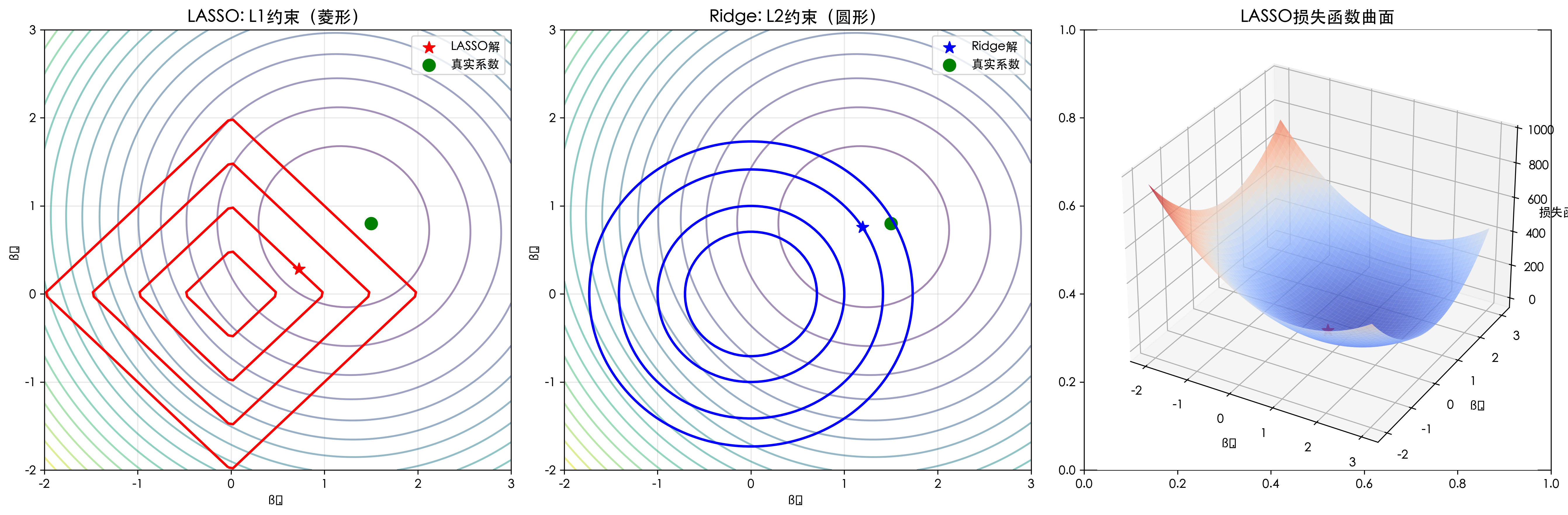

总结

LASSO的核心要点总结

稀疏性：LASSO的核心优势是产生稀疏解，自动进行特征选择
特征选择：通过L1正则化将不重要特征的系数压缩为0
参数选择：λ控制正则化强度，需要通过交叉验证选择
标准化：使用LASSO前必须对特征进行标准化
计算效率：坐标下降法可高效求解