从ResNet到mHC：DeepSeek重构残差连接，额外开销仅6.7%，附复现代码

关注公zh: AI-Frontiers

论文标题：mHC: Manifold-Constrained Hyper-Connections

论文地址：arxiv.org/pdf/2512.24...

延续在节假日搞事情的习惯，2026年元旦期间，Deepseek发表了一篇新论文，提出了名为mHC（Manifold-Constrained Hyper-Connections，流形约束超连接）的新架构。相信各位道友当时心里是五味陈杂：终于又可以抄作业了，等等，为啥你要元旦发啊，还让不让人过节啦。

该研究目标在不损失传统HC（超链接）性能增益的基础上，改善其在大模型训练过程中存在的不稳定性问题。

这次创新并非简单的组件替换，而是对神经网络宏观拓扑的一次重构。mHC将传统Transformer的单一残差流扩展为多流并行架构，通过引入严谨的几何流形约束，成功解决了HC在大规模训练中的数值不稳定和信号爆炸问题。

本文将带大家深扒这篇论文的提出背景、底层原理和实验效果，并附带网友的实战代码资源。

基本概念

残差连接

论文标题：Deep Residual Learning for Image Recognition

论文地址：arxiv.org/pdf/1512.03...

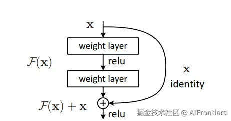
2015年，由微软亚洲研究院的何恺明团队提出ResNet，ResNet引入残差连接的概念，用以解决深层神经网络训练中的梯度消失/爆炸和网络退化问题，使得训练极深的网络成为可能。
<math xmlns="http://www.w3.org/1998/Math/MathML" display="block"> x l + 1 = x l + F ( x l , W l ) (1) \begin{align} x_{l+1} = x_l + F(x_l, W_l) \end{align} \tag {1} </math>xl+1=xl+F(xl,Wl)(1)

在公式（1）中：

<math xmlns="http://www.w3.org/1998/Math/MathML"> x l ∈ R 1 × d x_l \in R^{1 \times d} </math>xl∈R1×d为 <math xmlns="http://www.w3.org/1998/Math/MathML"> l l </math>l 层网络输入
<math xmlns="http://www.w3.org/1998/Math/MathML"> F F </math>F为对 <math xmlns="http://www.w3.org/1998/Math/MathML"> l l </math>l层进行的非线性变换，如卷积、Attention或MLP等
<math xmlns="http://www.w3.org/1998/Math/MathML"> x l + 1 ∈ R 1 × d x_{l+1} \in R^{1 \times d} </math>xl+1∈R1×d为该层的输出

传统的网络试图对每层的输入 <math xmlns="http://www.w3.org/1998/Math/MathML"> x x </math>x 直接学习目标映射 <math xmlns="http://www.w3.org/1998/Math/MathML"> H ( x ) H(x) </math>H(x)。而残差网络的设计思想是：既然直接学习很难，不如让网络去学习每层的残差，
<math xmlns="http://www.w3.org/1998/Math/MathML" display="block"> F ( x ) = H ( x ) − x (2) \begin{align} F(x) = H(x) - x \end{align} \tag {2} </math>F(x)=H(x)−x(2)

公式（1）和公式（2）本质是一样的：

公式（2）中的 <math xmlns="http://www.w3.org/1998/Math/MathML"> F ( x ) F(x) </math>F(x)即为公式（1）的 <math xmlns="http://www.w3.org/1998/Math/MathML"> F F </math>F
公式（2）中的 <math xmlns="http://www.w3.org/1998/Math/MathML"> H ( x ) H(x) </math>H(x)即为公式（1）的 <math xmlns="http://www.w3.org/1998/Math/MathML"> x l + 1 x_{l+1} </math>xl+1
公式（2）中的 <math xmlns="http://www.w3.org/1998/Math/MathML"> x x </math>x 即为公式（1）的 <math xmlns="http://www.w3.org/1998/Math/MathML"> x l x_l </math>xl

这就像是把原始文件 <math xmlns="http://www.w3.org/1998/Math/MathML"> x x </math>x复印了一份直接交给下一个人，同时附上一张便利贴，上面写着这一层所做的修改 <math xmlns="http://www.w3.org/1998/Math/MathML"> F ( x ) F(x) </math>F(x)。下一个人收到的是「原件 + 修改意见」，该设计的关键特性是恒等映射（Identity Mapping）能力。

在网络初始化的早期阶段，权重通常很小 <math xmlns="http://www.w3.org/1998/Math/MathML"> F ( x ) ≈ 0 F(x) \approx 0 </math>F(x)≈0。此时：
<math xmlns="http://www.w3.org/1998/Math/MathML" display="block"> x l + 1 ≈ x l + 0 = x l (3) \begin{align} x_{l+1} \approx x_l + 0 = x_l \end{align} \tag {3} </math>xl+1≈xl+0=xl(3)

这意味着，信号像是在高速公路上一样，毫无阻碍地从第一层直通最后一层。梯度也可以沿着这条高速公路无损地回传。正是这一特性，使得训练成百上千层的网络（如GPT-4, DeepSeek-V3）成为可能。

超连接（Hyper-Connections, HC）

论文标题：HYPER-CONNECTIONS

论文地址：arxiv.org/pdf/2409.19...

残差连接的问题

标准的残差连接强制要求输入信号与经过变换的信号以 1:1 的比例叠加，虽然保证了梯度的高速公路，但也带来了两个问题：

信息流瓶颈：原来只有一条残差通道，所有信息不管是简单细节还是高层抽象，都挤在同一条路上传。这就像所有车都走一条车道，没法灵活分配路线，模型没法根据需要把信息送到最合适的地方。
表示坍塌：网络特别深的时候，为了不崩、训练稳定，很多层其实学不到有用的新东西，只能改一点点、几乎等于没改。结果就是白白浪费算力，提取出来的特征都长得差不多，没有多样性，表达能力变弱。

在上面的背景下，字节提出了Hyper-Connections的模型结构来改进传统的残差连接结构。通过扩展残差流宽度和多样化连接模式，拓展了过去十年中广泛应用的残差连接范式。

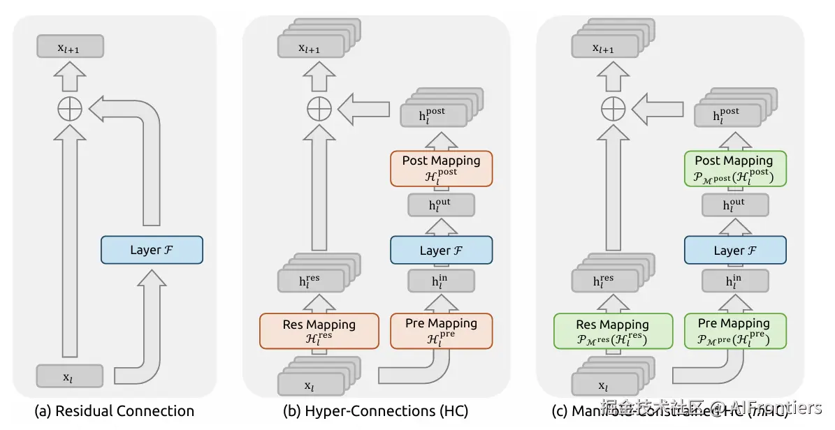
HC的核心思想是将原本单一维度的残差流扩展为$$$$个并行的流，然后乘以一个权重矩阵 <math xmlns="http://www.w3.org/1998/Math/MathML"> H l r e s H_l^{res} </math>Hlres。这增加了信息的带宽，可以更多地捕获输入不同维度之间的融合信息。

在HC架构中，信息不再是简单的标量加法，而是通过矩阵运算进行复杂的混合，数学表达为：
<math xmlns="http://www.w3.org/1998/Math/MathML" display="block"> x l + 1 = H l r e s x l + H l p o s t T F l ( H l p r e x l , W l ) (4) \begin{align} x_{l+1} = H_l^{res}x_l + H_l^{post \ T} F_{l}(H_l^{pre}x_l, W_l) \end{align} \tag {4} </math>xl+1=Hlresxl+Hlpost TFl(Hlprexl,Wl)(4)

对于公式（4）

<math xmlns="http://www.w3.org/1998/Math/MathML"> H p r e H^{pre} </math>Hpre （预融合/汇聚） ：将 <math xmlns="http://www.w3.org/1998/Math/MathML"> n n </math>n个并行流的信息汇聚起来，压缩成适合Transformer层（Attention或MLP）处理的输入维度。
<math xmlns="http://www.w3.org/1998/Math/MathML"> H p o s t H^{post} </math>Hpost （后融合/分发） ：将Transformer层的计算结果重新分发回 <math xmlns="http://www.w3.org/1998/Math/MathML"> n n </math>n个并行流中。
<math xmlns="http://www.w3.org/1998/Math/MathML"> H r e s H^{res} </math>Hres （流内混合） ：这是最激进也是最关键的组件。它允许 <math xmlns="http://www.w3.org/1998/Math/MathML"> n n </math>n个并行流在不经过Transformer层计算的情况下，直接进行内部的信息交换和混合。

理论上，HC允许模型学习出任意的连接模式：① 模型认为某一层应该保持恒等映射，可以学习将 <math xmlns="http://www.w3.org/1998/Math/MathML"> H r e s H^{res} </math>Hres变为单位矩阵 <math xmlns="http://www.w3.org/1998/Math/MathML"> I I </math>I；② 如果模型认为需要剧烈改变信息流向，可以学习复杂的非对角矩阵。这种灵活性极大地增强了模型的拓扑结构复杂度。

mHC

HC 的问题

根据公式（1），传统的残差连接结构模型第 <math xmlns="http://www.w3.org/1998/Math/MathML"> L L </math>L层和第 <math xmlns="http://www.w3.org/1998/Math/MathML"> l l </math>l层的关系表示如下：
<math xmlns="http://www.w3.org/1998/Math/MathML" display="block"> x L = x l + Σ i = l L − 1 F i ( x i , W i ) (5) \begin{align} x_L = x_l + \Sigma_{i=l}^{L-1} F_{i}(x_i, W_i) \end{align} \tag {5} </math>xL=xl+Σi=lL−1Fi(xi,Wi)(5)

上式表明 <math xmlns="http://www.w3.org/1998/Math/MathML"> x l x_l </math>xl的梯度信息可以1比1传递给 <math xmlns="http://www.w3.org/1998/Math/MathML"> x L x_L </math>xL，不会梯度爆炸或者梯度消失，保证训练过程的稳定性。

根据公式（4），可推导出HC结构下第 <math xmlns="http://www.w3.org/1998/Math/MathML"> L L </math>L层和第 <math xmlns="http://www.w3.org/1998/Math/MathML"> l l </math>l层的关系：
<math xmlns="http://www.w3.org/1998/Math/MathML" display="block"> x L = ( ∏ i = 1 L − 1 H L − i r e s ) x l + Σ i = l L − 1 ( ∏ j = 1 L − 1 − i H L − j r e s ) H i p o s t T F ( H i p r e x i , W i ) (6) \begin{align} x_L = (\prod_{i=1}^{L-1} H_{L-i}^{res}) \ x_l + \Sigma_{i=l}^{L-1} (\prod_{j=1}^{L-1-i} H_{L-j}^{res}) \ H_i^{post \ T} F(H_i^{pre} x_i, W_i) \end{align} \tag {6} </math>xL=(i=1∏L−1HL−ires) xl+Σi=lL−1(j=1∏L−1−iHL−jres) Hipost TF(Hiprexi,Wi)(6)

这会导致 <math xmlns="http://www.w3.org/1998/Math/MathML"> ∂ l o s s ∂ x L ( ∏ i = 1 L − 1 H L − i r e s ) ∂ l o s s ∂ x l + . . . \frac{\partial loss}{\partial x_L} (\prod_{i=1}^{L-1} H_{L-i}^{res}) \frac{\partial loss}{\partial x_l} + ... </math>∂xL∂loss(∏i=1L−1HL−ires)∂xl∂loss+...。由于 <math xmlns="http://www.w3.org/1998/Math/MathML"> ∏ i = 1 L − 1 H L − i r e s \prod_{i=1}^{L-1} H_{L-i}^{res} </math>∏i=1L−1HL−ires一个典型的连乘过程，矩阵连乘的性质取决于矩阵的谱范数，即矩阵最大特征值的模。我们来比较Resnet中残差连接和HC连乘的情况：

Resnet中的残差连接 ：残差路径是恒等映射，相当于乘以单位矩阵 <math xmlns="http://www.w3.org/1998/Math/MathML"> I I </math>I。单位矩阵的谱范数严格为 1。无论乘多少次， <math xmlns="http://www.w3.org/1998/Math/MathML"> 1 100 = 1 1^{100} = 1 </math>1100=1，信号始终稳定。
HC ：在HC中， <math xmlns="http://www.w3.org/1998/Math/MathML"> H r e s H^{res} </math>Hres是自由学习的参数矩阵，不可控。
- 如果 <math xmlns="http://www.w3.org/1998/Math/MathML"> H r e s H^{res} </math>Hres的平均谱范数略大于 1（例如 1.05），在 60 层的网络中，信号会被放大 <math xmlns="http://www.w3.org/1998/Math/MathML"> 1.0 5 60 ≈ 18.6 1.05^{60} \approx 18.6 </math>1.0560≈18.6倍。
- 如果谱范数更大，或者网络更深，放大倍数会呈指数级爆炸，破坏残差结构中梯度回传的稳定性，从而导致训练不稳定，具体可见下图。

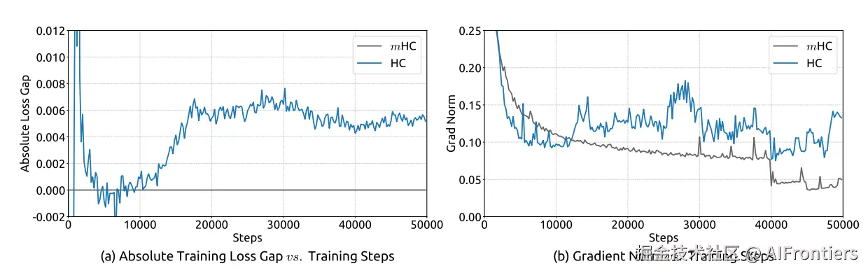
上图显示，27B模型训练到12k step左右，HC的loss突然飙升。与此同时，梯度范数也开始疯狂震荡。

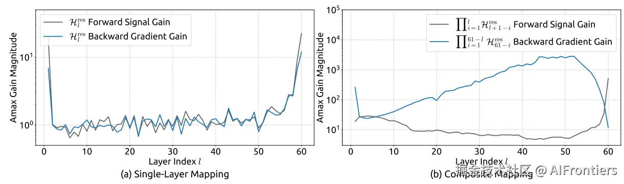
另外，由于 <math xmlns="http://www.w3.org/1998/Math/MathML"> H L − i r e s H_{L-i}^{res} </math>HL−ires矩阵是无约束的，可以往任意方向发散。论文测量了一个叫「Amax Gain Magnitude」的指标，在残差流里被放大了3000倍。在大规模训练中，这就是爆炸的前奏。

mHC的诞生

面对HC的问题，DeepSeek提出了mHC，即Manifold-Constrained Hyper-Connections（流形约束超连接），其核心思路为：将不可控的 <math xmlns="http://www.w3.org/1998/Math/MathML"> H r e s H^{res} </math>Hres矩阵通过数学的手段，转换为可控的双随机矩阵（Doubly Stochastic Matrices）。下面为大家解释mHC几个重要概念。

双随机矩阵（Doubly Stochastic Matrices）

双随机矩阵定义如下：
<math xmlns="http://www.w3.org/1998/Math/MathML" display="block"> P M res ( H l res ) : = { H l res ∈ R n × n ∣ H l res 1 n = 1 n , 1 n ⊤ H l res = 1 n ⊤ , H l res ≥ 0 } (7) \begin{align} \mathcal{P}{\mathcal{M}^{\text{res}}}\left(\mathcal{H}{l}^{\text{res}}\right) := \left\{ \mathcal{H}{l}^{\text{res}} \in \mathbb{R}^{n \times n} \mid \mathcal{H}{l}^{\text{res}} \mathbf{1}_n = \mathbf{1}_n,\ \mathbf{1}n^\top \mathcal{H}{l}^{\text{res}} = \mathbf{1}n^\top,\ \mathcal{H}{l}^{\text{res}} \ge 0 \right\} \end{align} \tag {7} </math>PMres(Hlres):={Hlres∈Rn×n∣Hlres1n=1n, 1n⊤Hlres=1n⊤, Hlres≥0}(7)

其中， <math xmlns="http://www.w3.org/1998/Math/MathML"> 1 n 1^n </math>1n表示所有元素均为 1 的 <math xmlns="http://www.w3.org/1998/Math/MathML"> n n </math>n维向量。从公式（7）中可看出，双随机矩阵的元素都大于等于0，每一行、每一列的值相加都等于1。

双随机矩阵具备2个重要特性：① 范数值为1；②多个双随机矩阵的乘积还是双随机矩阵。从而可以推出 <math xmlns="http://www.w3.org/1998/Math/MathML"> ∣ ∏ i = 1 L − 1 H L − i r e s ∣ = 1 |\prod_{i=1}^{L-1} H_{L-i}^{res}| = 1 </math>∣∏i=1L−1HL−ires∣=1 ，解决了上面提到的范数不可控的问题。

那么怎么把 <math xmlns="http://www.w3.org/1998/Math/MathML"> H l r e s H^{res}_l </math>Hlres矩阵变换成双随机矩阵呢？DeepSeek团队采用的是Sinkhorn-Knopp算法。

Sinkhorn-Knopp算法

① 通过公式（8）计算变换前的 <math xmlns="http://www.w3.org/1998/Math/MathML"> H l r e s H^{res}_l </math>Hlres：
<math xmlns="http://www.w3.org/1998/Math/MathML" display="block"> { x ~ l ′ = RMSNorm ( x ~ l ) H ~ l pre = α l pre ⋅ ( x ~ l ′ φ l pre ) + b l pre H ~ l post = α l post ⋅ ( x ~ l ′ φ l post ) + b l post H ~ l res = α l res ⋅ mat ( x ~ l ′ φ l res ) + b l res , (8) \begin{align} \begin{cases} \tilde{x}_l' = \text{RMSNorm}(\tilde{x}_l) \\ \tilde{\mathcal{H}}_l^{\text{pre}} = \alpha_l^{\text{pre}} \cdot \left( \tilde{x}_l' \varphi_l^{\text{pre}} \right) + \mathbf{b}_l^{\text{pre}} \\ \tilde{\mathcal{H}}_l^{\text{post}} = \alpha_l^{\text{post}} \cdot \left( \tilde{x}_l' \varphi_l^{\text{post}} \right) + \mathbf{b}_l^{\text{post}} \\ \tilde{\mathcal{H}}_l^{\text{res}} = \alpha_l^{\text{res}} \cdot \text{mat}(\tilde{x}_l' \varphi_l^{\text{res}}) + \mathbf{b}_l^{\text{res}}, \end{cases} \end{align} \tag {8} </math>⎩ ⎨ ⎧x~l′=RMSNorm(x~l)H~lpre=αlpre⋅(x~l′φlpre)+blpreH~lpost=αlpost⋅(x~l′φlpost)+blpostH~lres=αlres⋅mat(x~l′φlres)+blres,(8)

其中，输入 <math xmlns="http://www.w3.org/1998/Math/MathML"> x l ∈ R n × C , φ l pre , φ l post ∈ R n C × n , φ l r e s ∈ R n C , n 2 {x}_l \in \mathbb{R}^{n \times C}, \varphi_l^{\text{pre}}, \varphi_l^{\text{post}} \in \mathbb{R}^{nC \times n}, \quad \varphi_l^{res} \in \mathbb{R}^{nC, n^2} </math>xl∈Rn×C,φlpre,φlpost∈RnC×n,φlres∈RnC,n2，先将 <math xmlns="http://www.w3.org/1998/Math/MathML"> x l {x}_l </math>xl转换为 <math xmlns="http://www.w3.org/1998/Math/MathML"> R 1 × n C {R}^{1 \times nC} </math>R1×nC的向量 <math xmlns="http://www.w3.org/1998/Math/MathML"> x ~ l \tilde{x}_l </math>x~l，并通过mat(·)操作从 <math xmlns="http://www.w3.org/1998/Math/MathML"> R 1 × n 2 {R}^{1 \times n^2} </math>R1×n2空间转换到 <math xmlns="http://www.w3.org/1998/Math/MathML"> R n × n {R}^{n \times n} </math>Rn×n。

② 通过 <math xmlns="http://www.w3.org/1998/Math/MathML"> M ( 0 ) = e x p ( H ~ l r e s ) M^{(0)} = exp\big(\tilde{H}_l^{res}\big) </math>M(0)=exp(H~lres)得到元素值都大于0的矩阵，作为迭代起始矩阵。

③ 通过下面的公式迭代做normalization，使其满足每行之和和每列之和接近1：
<math xmlns="http://www.w3.org/1998/Math/MathML" display="block"> M ( t ) = T r ( T c ( M ( t − 1 ) ) ) (9) \begin{align} \mathbf{M}^{(t)} = \mathcal{T}_r\big(\mathcal{T}_c(\mathbf{M}^{(t-1)})\big) \end{align} \tag {9} </math>M(t)=Tr(Tc(M(t−1)))(9)

其中 <math xmlns="http://www.w3.org/1998/Math/MathML"> T r \mathcal{T}_r </math>Tr 和 <math xmlns="http://www.w3.org/1998/Math/MathML"> T c \mathcal{T}_c </math>Tc分别代表按行和按列做归一化，根据Sinkhorn-Knopp算法原理， <math xmlns="http://www.w3.org/1998/Math/MathML"> M ( t ) \mathbf{M}^{(t)} </math>M(t)会收敛成双随机矩阵，DeepSeek论文中一般迭代20步。

Birkhoff多胞体 流形

论文标题中的Manifold（流形）指的就是由所有双随机矩阵构成的几何空间，被称为Birkhoff多胞体（Birkhoff Polytope）, 记为 <math xmlns="http://www.w3.org/1998/Math/MathML"> B n \mathcal{B}_n </math>Bn。

多胞体（Polytope） ：想象一个多维空间中的多面体（类似于3D空间中的钻石或立方体）。这个多面体的每一个点，都代表一个合法的双随机矩阵。
顶点（Vertices） ：这个多面体的顶点是所有的置换矩阵（Permutation Matrices）。置换矩阵是只包含0和1的矩阵，且每行每列只有一个1。它们的作用仅仅是交换信息的顺序（比如把通道1的信息换到通道 2），而不改变信息的大小。
内部（Interior） ：Birkhoff-von Neumann定理告诉我们，这个多面体内部的任何一个点（即任何一个双随机矩阵），都可以表示为这些顶点的加权平均。

DeepSeek的做法，实际上是将神经网络原本在整个欧几里得空间中乱跑的参数，强行拉回到了这个 Birkhoff多胞体的表面或内部。在这个几何体内游走，无论怎么走，都是安全的。

关于mHC的更多知识，可参考www.k-a.in/mHC-math.ht...

系统级实现与工程优化

虽然Sinkhorn-Knopp迭代在理论上很美，但在计算上却很昂贵。如果在每一层、每一步训练中都进行 20次矩阵迭代，训练速度会大打折扣。DeepSeek为mHC量身定制了基础设施设计，将额外开销仅增加6.7%。

算子融合 (Kernel Fusion)

DeepSeek利用了自研的TileLang编程语言开发了定制化的CUDA内核。

融合操作：将指数化、20次Sinkhorn迭代、以及后续的矩阵乘法，全部融合进了一个单一的GPU Kernel中。
SRAM 驻留：在这个Kernel执行期间，中间数据（如迭代过程中的矩阵）一直保留在GPU的高速缓存（SRAM/Register）中，而不需要反复写回慢速的全局显存。

这大大减少了内存 I/O 次数，使得 20 次迭代的计算时间几乎可以忽略不计。

DualPipe通信重叠

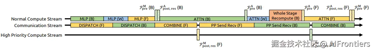
在大模型训练中，由于模型太大，往往需要跨多个GPU进行流水线并行（Pipeline Parallelism）。 DeepSeek设计了一种名为DualPipe的调度策略。

打时间差：当GPU的计算单元（Tensor Cores）正在全力计算mHC的Sinkhorn投影时，GPU的通信单元（NVLink）并未闲着。
重叠执行：DualPipe巧妙地安排了任务，利用mHC计算的时间窗口，同时进行不同GPU之间的数据传输。
结果：Sinkhorn带来的额外计算延迟被通信时间完美掩盖了。对于整体训练流程来说，mHC的计算几乎是免费的。

选择性重计算（Selective Recomputation）

由于mHC引入了 <math xmlns="http://www.w3.org/1998/Math/MathML"> n = n= </math>n= 的扩展流，中间激活值的显存占用会增加。如果全部存储，会导致显存不足。

DeepSeek 采用了选择性重计算策略：

在前向传播时，不存储所有Sinkhorn迭代的中间结果。
在反向传播时，利用这一层极快的计算速度，重新计算出所需的中间变量。
这种以计算换显存的策略，结合TileLang的高效率，使得 mHC 在显存占用上也保持了高效。

实验结果

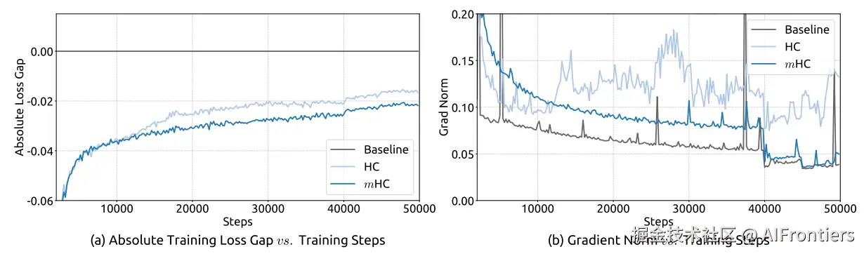
研究首先考察27B模型的训练稳定性与收敛性。如图5 (a) 所示，mHC有效缓解了在HC中观察到的训练不稳定性，与基线相比，最终损失降低了0.021。图5 (b) 中的梯度范数分析进一步证实了这种稳定性的提升，其中mHC表现出明显优于HC的行为，其稳定的表现与基线相当。

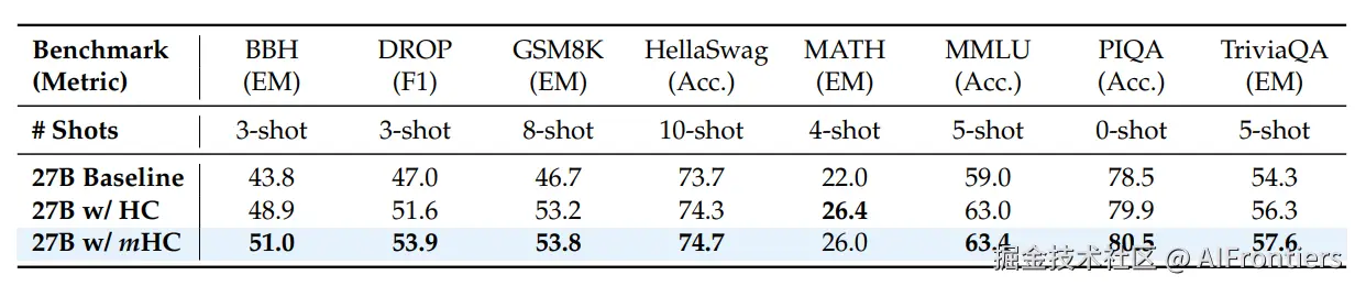
表 4展示了模型在多种下游基准测试中的性能表现。相比于基线模型，mHC实现了全面的性能提升，并在大多数任务上超过了HC。值得注意的是，与HC相比，mHC 进一步增强了模型的推理能力，在 BBH上实现了2.1%的性能提升，在 DROP上实现了2.3%的性能提升。

代码实现

github网友实现的代码，仅供参考

参考资料

arxiv.org/pdf/2512.24...

arxiv.org/pdf/2409.19...

arxiv.org/pdf/1512.03...

Deriving Manifold Constrained Hyper Connections