MATLAB学习笔记------第五章
| 问题类型 | 函数 |
|---|---|
| 显式微分方程 | ode23/ode113 |
| 完全隐式微分方程 | ode15i |
| 代数微分方程显式 | ode15s |
| 代数微分方程隐式 | ode15i |
| 延迟微分方程 | dde23 |
显式微分方程
刚性方程与非刚性方程的直接判别方法就是从解在某段时间区间内的变化来看,非刚性问题变化相对缓慢,刚性问题在某段时间内发生剧烈变化

matlab
figure(1)
tspan = 0:10;						% 求解区间
y0 = 2;
sol1 = ode23(@odefun1,tspan,y0);     % 数值解
sol2 = ode113(@odefun1,tspan,y0);    % 数值解
% deval :计算微分方程区间内任意点的值
ts = 0:10;
y1 = deval(sol1,ts);
y2 = deval(sol2,ts);                 % 此时y1,y2均为11个值

yt = sqrt(ts+1)+1;              	 % 精确解
subplot(1,2,1)
plot(ts,yt,'r-','linewidth',1.5)
grid on;	hold on;
plot(ts,y1,'bo',ts,y2,'k*')
legend('精确值曲线','ode23点','ode113点')
hold off

subplot(1,2,2)
y1t = abs(yt-y1);
y2t = abs(yt-y2);
plot(ts,y1t,'ro',ts,y2t,'bo')
legend('ode23误差','ode113误差')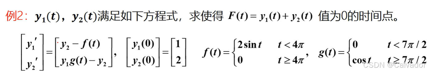
matlab
figure(2)
ts = [0,20];	% 求解区间
y0 = [1,2];		% 初始解
sol = ode23tb(@odefun2,ts,y0);	% 刚性方程
subplot(1,2,1)
plot(sol.x,sol.y(1,:),'b-','linewidth',1.5)
hold on;	grid on;
plot(sol.x,sol.y(2,:),'r--','linewidth',1.5)
legend('{\ity}_1(t)','{\ity}_2(t)','Location','best')
hold off

subplot(1,2,2)
ysum = sum(sol.y);
% 为了使用fzero函数,因此通过画图找初值
plot(sol.x,ysum,'b-','linewidth',1.5)
hold on;    grid on
fplot(@(t)0*t,[0,20])
hold off
fh = @(t)sum(deval(sol,t));
y01 = fzero(fh,10);
完全隐式微分方程
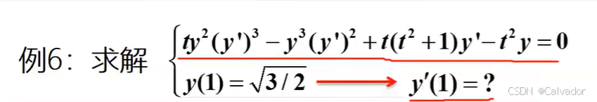
matlab
figure(3)
y0 = sqrt(3/2);
yp0 = 0.5;  % 猜测
t0 = 1;
% decic:用于求解y0已知的时候的yp0的初值
[y0mod,yp0mod] = decic(@odefun3,t0,y0,1,yp0,0);
[t,y] = ode15i(@weissinger,[1 10],y0,yp0);
ytrue = sqrt(t.^2 + 0.5);
plot(t,y,'*',t,ytrue,'-o')
legend('ode15i求解', '精确解','Location','best')
legend('boxoff')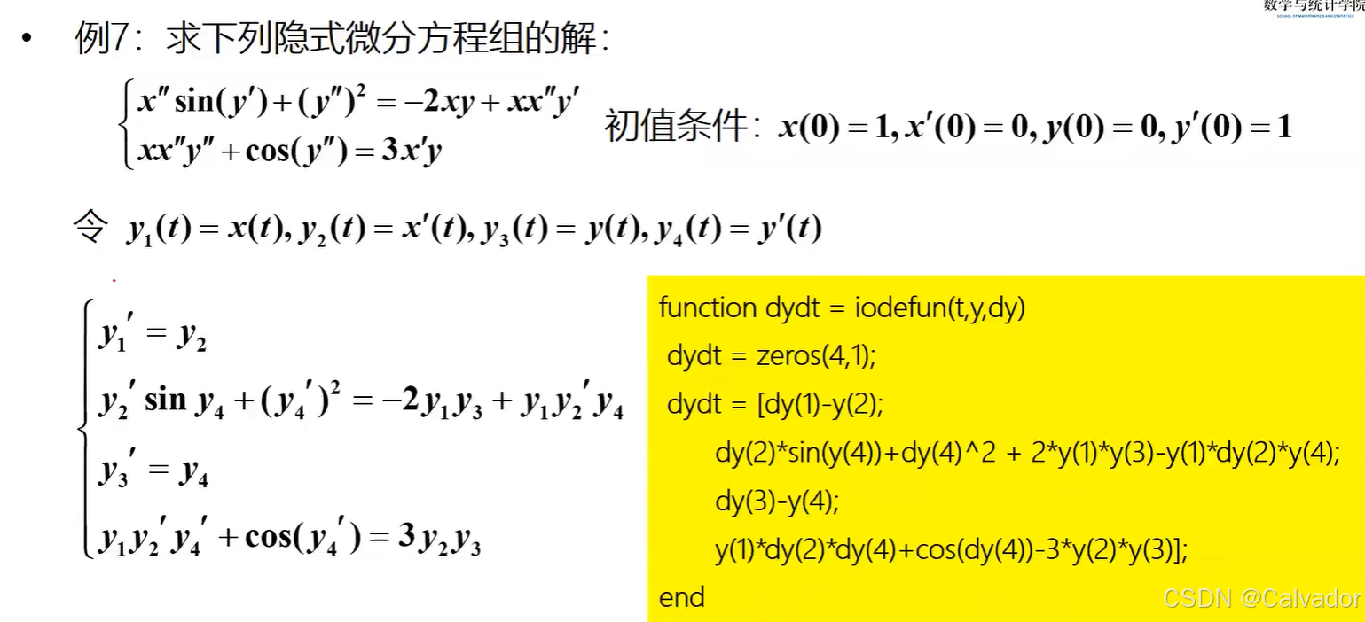
matlab
figure(4)
t0 = 0;
y0 = [1;0;0;1];
fix_y0 = ones(4,1);
fix_yp0 = zeros(4,1);
yp0 = [0;2;1;-0.5];
[y02,yp02] = decic(@odefun4,t0,y0,fix_y0,yp0,fix_yp0);
[t,y] = ode15i(@odefun4,[0,5],y0,yp02);
plot(t,y(:,1),'r-',t,y(:,2),'b--',t,y(:,3),'c.-',t,y(:,4),'k:','LineWidth',1.5)
legend('y1','y2','y3','y4','Location','best')
grid on
代数微分方程
显式
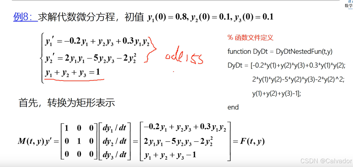
matlab
figure(5)
y0 = [0.8,0.1,0.1]';
M = eye(3); M(3,3)=0;
options = odeset('Mass',M,'RelTol',1e-4,'AbsTol',[1e-6 1e-10 1e-6]);
[t,y] = ode15s(@odefun5,[0,20],y0,options);
plot(t,y(:,1),'r--',t,y(:,2),'b.-',t,y(:,3),'k:','LineWidth',1.5)
legend('y1','y2','y3','Location','best')
grid on
隐式
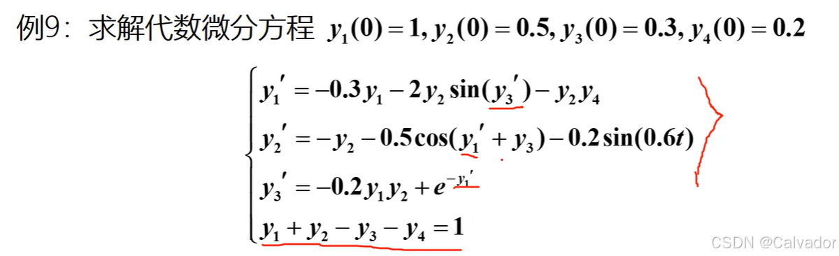
matlab
figure(6)
y0 = [1;0.5;0.3;0.2];
% 首先通过decic函数求yp0,使得f(t,y,yp) = 0
t0 = 0;
fix_y0 = [0;1;1;1];
fix_yp0 = zeros(4,1);
yp0 = [-0.8;-1;1;1];    % 猜测
[y02,yp02] = decic(@odefun6,t0,y0,fix_y0,yp0,fix_yp0);
[t,y] = ode15i(@odefun6,[0,10],y0,yp02);
plot(t,y(:,1),'r--',t,y(:,2),'b.-',t,y(:,3),'k:',t,y(:,4),'c','LineWidth',1.5)
legend('y1','y2','y3','y4','Location','best')
grid on
延迟微分方程
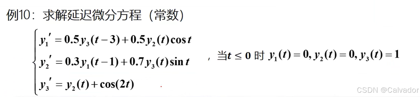
matlab
lags = [1,3];   % 延迟常数向量
history = [0,0,1];  % 小于t0时刻的历史函数
tspan = [0,8];
sol = dde23(@odefun7,lags,history,tspan);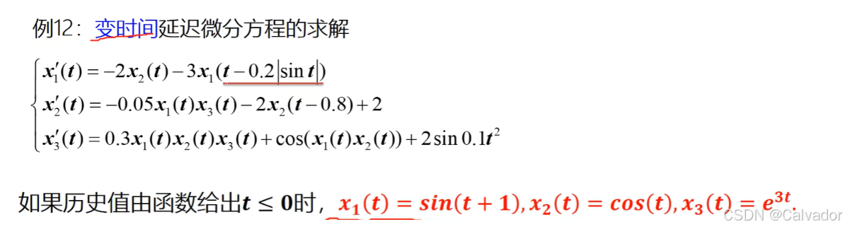
matlab
figure(7)
lags = @(t,x)[t-0.2*abs(sin(t));t-0.8];
% history = zeros(3,1);   % 未给的情况
history = @(t,x)[sin(t+1); cos(t); exp(3*t)];
tspan = [0,10];
sol = ddesd(@odefun8,lags,history,tspan);
plot(sol.x,sol.y(1,:),sol.x,sol.y(2,:),sol.x,sol.y(3,:),'LineWidth',1.5)