CART决策树基本原理

分类与回归树(classification and regression tree, CART)模型由特征选择、树的生成及剪枝组成，既可以用于分类也可以用于回归。

以下将用于分类与回归的树统称为决策树。CART是在给定输入随机变量 <math xmlns="http://www.w3.org/1998/Math/MathML"> X X </math>X条件下输出随机变量 <math xmlns="http://www.w3.org/1998/Math/MathML"> Y Y </math>Y的条件概率分布的学习方法。CART假设决策树是二叉树，内部结点特征的取值为"是"和"否"​，左分支是取值为"是"的分支，右分支是取值为"否"的分支。这样的决策树等价于递归地二分每个特征，将输入空间即特征空间划分为有限个单元，并在这些单元上确定预测的概率分布，也就是在输入给定的条件下输出的条件概率分布。

CART算法由以下两步组成：

1. 决策树生成：基于训练数据集生成决策树，生成的决策树要尽量大；
2. 决策树剪枝：用验证数据集对已生成的树进行剪枝并选择最优子树，这时用损失函数最小作为剪枝的标准。

CART生成

决策树的生成就是递归地构建二叉决策树的过程。对回归树用平方误差最小化准则，对分类树用基尼指数(Gini index)最小化准则，进行特征选择，生成二叉树。

分类树

分类树用基尼不纯度和基尼指数选择最优特征，同时决定该特征的最优二值切分点。

基尼不纯度

分类问题中，假设有 <math xmlns="http://www.w3.org/1998/Math/MathML"> K K </math>K个类，样本点属于第 <math xmlns="http://www.w3.org/1998/Math/MathML"> k k </math>k类的概率为 <math xmlns="http://www.w3.org/1998/Math/MathML"> p k p_k </math>pk，则概率分布的基尼不纯度(Gini impurity)定义为
<math xmlns="http://www.w3.org/1998/Math/MathML" display="block"> G ( p ) = ∑ k = 1 K p k ( 1 − p k ) = 1 − ∑ k = 1 K p k 2 \begin{equation} G(p)=\sum_{k=1}^Kp_k(1-p_k)=1-\sum_{k=1}^Kp_k^2 \end{equation} </math>G(p)=k=1∑Kpk(1−pk)=1−k=1∑Kpk2

对于二类分类问题，若样本点属于第1个类的概率是 <math xmlns="http://www.w3.org/1998/Math/MathML"> p p </math>p，则概率分布的基尼不纯度为
<math xmlns="http://www.w3.org/1998/Math/MathML" display="block"> G ( p ) = 2 p ( 1 − p ) \begin{equation} G(p)=2p(1-p) \end{equation} </math>G(p)=2p(1−p)

对于给定的样本集合 <math xmlns="http://www.w3.org/1998/Math/MathML"> D D </math>D，其基尼不纯度为
<math xmlns="http://www.w3.org/1998/Math/MathML" display="block"> G ( D ) = 1 − ∑ k = 1 K ( ∣ C k ∣ ∣ D ∣ ) 2 \begin{equation} G(D)=1-\sum_{k=1}^K\left(\frac{|C_k|}{|D|}\right)^2 \end{equation} </math>G(D)=1−k=1∑K(∣D∣∣Ck∣)2

这里， <math xmlns="http://www.w3.org/1998/Math/MathML"> C k C_k </math>Ck是 <math xmlns="http://www.w3.org/1998/Math/MathML"> D D </math>D中属于第 <math xmlns="http://www.w3.org/1998/Math/MathML"> k k </math>k类的样本子集， <math xmlns="http://www.w3.org/1998/Math/MathML"> K K </math>K是类的个数。基尼不纯度 <math xmlns="http://www.w3.org/1998/Math/MathML"> G ( D ) G(D) </math>G(D)表示集合 <math xmlns="http://www.w3.org/1998/Math/MathML"> D D </math>D的不确定性。

基尼增益

如果样本集合 <math xmlns="http://www.w3.org/1998/Math/MathML"> D D </math>D根据特征 <math xmlns="http://www.w3.org/1998/Math/MathML"> A A </math>A是否取某一可能值 <math xmlns="http://www.w3.org/1998/Math/MathML"> a a </math>a被分割成 <math xmlns="http://www.w3.org/1998/Math/MathML"> D 1 D_1 </math>D1和 <math xmlns="http://www.w3.org/1998/Math/MathML"> D 2 D_2 </math>D2两部分，即
<math xmlns="http://www.w3.org/1998/Math/MathML" display="block"> D 1 = { ( x , y ) ∈ D ∣ A ( x ) = a } D 2 = { ( x , y ) ∈ D ∣ A ( x ) ≠ a } \begin{equation} \begin{aligned} D_1=\{(x,y)\in D|A(x)=a\}\\ D_2=\{(x,y)\in D|A(x)\not=a\} \end{aligned} \end{equation} </math>D1={(x,y)∈D∣A(x)=a}D2={(x,y)∈D∣A(x)=a}

基尼不纯度 <math xmlns="http://www.w3.org/1998/Math/MathML"> G ( D 1 ) G(D_1) </math>G(D1)和 <math xmlns="http://www.w3.org/1998/Math/MathML"> G ( D 2 ) G(D_2) </math>G(D2)分别根据子集合 <math xmlns="http://www.w3.org/1998/Math/MathML"> D 1 D_1 </math>D1和 <math xmlns="http://www.w3.org/1998/Math/MathML"> D 2 D_2 </math>D2里的样本情况进行计算。集合 <math xmlns="http://www.w3.org/1998/Math/MathML"> D , D 1 , D 2 D,D_1,D_2 </math>D,D1,D2中的样本数量分别用 <math xmlns="http://www.w3.org/1998/Math/MathML"> ∣ D ∣ , ∣ D 1 ∣ , ∣ D 2 ∣ |D|,|D_1|,|D_2| </math>∣D∣,∣D1∣,∣D2∣表示，则根据属性 <math xmlns="http://www.w3.org/1998/Math/MathML"> A A </math>A的值 <math xmlns="http://www.w3.org/1998/Math/MathML"> a a </math>a进行划分时，所获得的基尼增益(Gini gain)的计算公式如下：
<math xmlns="http://www.w3.org/1998/Math/MathML" display="block"> G G ( A = a ) = G ( D ) − ∣ D 1 ∣ ∣ D ∣ G ( D 1 ) − ∣ D 2 ∣ ∣ D ∣ G ( D 2 ) \begin{equation} GG(A=a)=G(D)-\frac{|D_1|}{|D|}G(D_1)-\frac{|D_2|}{|D|}G(D_2) \end{equation} </math>GG(A=a)=G(D)−∣D∣∣D1∣G(D1)−∣D∣∣D2∣G(D2)

基尼指数

在针对节点进行属性和分割点的选择时，面对的是同一个数据集合 <math xmlns="http://www.w3.org/1998/Math/MathML"> D D </math>D，这个集合可能是最初的完整数据集合，也可能是经过分割后形成的子集合。但无论哪种情况， <math xmlns="http://www.w3.org/1998/Math/MathML"> G ( D ) G(D) </math>G(D)都是相同的，因此可以对基尼增益的计算公式进行变换，得到基尼指数(Gini index)​，它的计算公式如下：
<math xmlns="http://www.w3.org/1998/Math/MathML" display="block"> G I ( D ) = ∣ D 1 ∣ D G ( D 1 ) + ∣ D 2 ∣ D G ( D 2 ) \begin{equation} GI(D)=\frac{|D_1|}{D}G(D_1)+\frac{|D_2|}{D}G(D_2) \end{equation} </math>GI(D)=D∣D1∣G(D1)+D∣D2∣G(D2)

基尼指数 <math xmlns="http://www.w3.org/1998/Math/MathML"> G I ( D , A ) GI(D,A) </math>GI(D,A)表示经 <math xmlns="http://www.w3.org/1998/Math/MathML"> A = a A=a </math>A=a分割后集合 <math xmlns="http://www.w3.org/1998/Math/MathML"> D D </math>D的不确定性，反映了从数据集 <math xmlns="http://www.w3.org/1998/Math/MathML"> D D </math>D中随机抽取两个样本，其类别标记不一致的概率。基尼指数值越小，样本集合的不确定性也就越小，做出的分割就越好，这一点与熵相似。

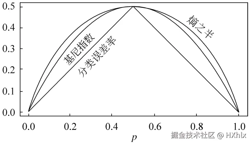
下图显示二类分类问题中基尼指数 <math xmlns="http://www.w3.org/1998/Math/MathML"> G I ( D ) GI(D) </math>GI(D)​、熵（单位比特）之半 <math xmlns="http://www.w3.org/1998/Math/MathML"> H ( p ) 2 \frac{H(p)}{2} </math>2H(p)和分类误差率的关系。横坐标表示概率 <math xmlns="http://www.w3.org/1998/Math/MathML"> p p </math>p，纵坐标表示损失。可以看出基尼指数和熵之半的曲线很接近，都可以近似地代表分类误差率。

CART分类树生成算法

输入：训练数据集 <math xmlns="http://www.w3.org/1998/Math/MathML"> D D </math>D，停止计算的条件。

输出：CART分类树。

根据训练数据集，从根结点开始，递归地对每个结点进行以下操作，构建二叉分类树：

1. 设结点的训练数据集为 <math xmlns="http://www.w3.org/1998/Math/MathML"> D D </math>D，计算现有特征对该数据集的基尼指数。此时，对每一个特征 <math xmlns="http://www.w3.org/1998/Math/MathML"> A A </math>A，对其可能取的每个值 <math xmlns="http://www.w3.org/1998/Math/MathML"> a a </math>a，根据样本点对 <math xmlns="http://www.w3.org/1998/Math/MathML"> A = a A=a </math>A=a的测试为"是"或"否"将 <math xmlns="http://www.w3.org/1998/Math/MathML"> D D </math>D分割成 <math xmlns="http://www.w3.org/1998/Math/MathML"> D 1 D_1 </math>D1和 <math xmlns="http://www.w3.org/1998/Math/MathML"> D 2 D_2 </math>D2两部分，利用式(6)计算 <math xmlns="http://www.w3.org/1998/Math/MathML"> A = a A=a </math>A=a时的基尼指数。
2. 在所有可能的特征 <math xmlns="http://www.w3.org/1998/Math/MathML"> A A </math>A以及它们所有可能的切分点 <math xmlns="http://www.w3.org/1998/Math/MathML"> a a </math>a中，选择基尼指数最小的特征及其对应的切分点作为最优特征与最优切分点。依最优特征与最优切分点，从现结点生成两个子结点，将训练数据集依特征分配到两个子结点中去。
3. 对两个子结点递归地调用步骤1和2，直至满足停止条件。
4. 生成CART决策树。

算法停止计算的条件是结点中的样本个数小于预定阈值，或样本集的基尼指数小于预定阈值（样本基本属于同一类）​，或者没有更多特征。

回归树

假设 <math xmlns="http://www.w3.org/1998/Math/MathML"> X X </math>X与 <math xmlns="http://www.w3.org/1998/Math/MathML"> Y Y </math>Y分别为输入和输出变量，并且 <math xmlns="http://www.w3.org/1998/Math/MathML"> Y Y </math>Y是连续变量，给定训练数据集 <math xmlns="http://www.w3.org/1998/Math/MathML"> D = { ( x i , y i ) } i = 1 N D=\{(x_i,y_i)\}_{i=1}^N </math>D={(xi,yi)}i=1N考虑如何生成回归树。

一棵回归树对应着输入空间（即特征空间）的一个划分以及在划分的单元上的输出值。假设已将输入空间划分为 <math xmlns="http://www.w3.org/1998/Math/MathML"> M M </math>M个单元 <math xmlns="http://www.w3.org/1998/Math/MathML"> R m , m = 1 , 2 , ⋯   , M R_m,m=1,2,\cdots,M </math>Rm,m=1,2,⋯,M，并且在每个单元 <math xmlns="http://www.w3.org/1998/Math/MathML"> R m R_m </math>Rm上有一个固定的输出值 <math xmlns="http://www.w3.org/1998/Math/MathML"> c m c_m </math>cm，于是回归树模型可表示为
<math xmlns="http://www.w3.org/1998/Math/MathML" display="block"> f ( x ) = ∑ m = 1 M c m I ( x ∈ R m ) \begin{equation} f(x)=\sum_{m=1}^Mc_mI(x\in R_m) \end{equation} </math>f(x)=m=1∑McmI(x∈Rm)

当输入空间的划分确定时，可以用平方误差
<math xmlns="http://www.w3.org/1998/Math/MathML" display="block"> 1 n ∑ m = 1 M ∑ x i ∈ R m ( y i − f ( x i ) ) 2 \frac{1}{n}\sum_{m=1}^M\sum_{x_i\in R_m}(y_i-f(x_i))^2 </math>n1m=1∑Mxi∈Rm∑(yi−f(xi))2

来表示回归树对于训练数据的预测误差，用平方误差最小的准则求解每个单元上的最优输出值。

问题是怎样对输入空间进行划分。这里采用启发式的方法，选择第 <math xmlns="http://www.w3.org/1998/Math/MathML"> j j </math>j个变量 <math xmlns="http://www.w3.org/1998/Math/MathML"> x ( j ) x^{(j)} </math>x(j)和它取的值 <math xmlns="http://www.w3.org/1998/Math/MathML"> s s </math>s，作为切分变量(splitting variable)和切分点(splitting point)​，并定义两个区域：
<math xmlns="http://www.w3.org/1998/Math/MathML" display="block"> R 1 ( j , s ) = { x ∣ x ( j ) ≤ s } R 2 ( j , s ) = { x ∣ x ( j ) > s } \begin{equation} \begin{aligned} R_1(j,s)=\{x|x^{(j)}\le s\}\\ R_2(j,s)=\{x|x^{(j)}>s\} \end{aligned} \end{equation} </math>R1(j,s)={x∣x(j)≤s}R2(j,s)={x∣x(j)>s}

然后寻找最优切分变量 <math xmlns="http://www.w3.org/1998/Math/MathML"> j j </math>j和最优切分点 <math xmlns="http://www.w3.org/1998/Math/MathML"> s s </math>s。具体地，求解
<math xmlns="http://www.w3.org/1998/Math/MathML" display="block"> min ⁡ j , s [ min ⁡ c 1 ∑ x i ∈ R 1 ( j , s ) ( y i − c 1 ) 2 + min ⁡ c 2 ∑ x i ∈ R 2 ( j , s ) ( y i − c 2 ) 2 ] \begin{equation} \min_{j,s}\left[\min_{c_1}\sum_{x_i\in R_1(j,s)}(y_i-c_1)^2+\min_{c_2}\sum_{x_i\in R_2(j,s)}(y_i-c_2)^2\right] \end{equation} </math>j,smin c1minxi∈R1(j,s)∑(yi−c1)2+c2minxi∈R2(j,s)∑(yi−c2)2

对固定输入变量 <math xmlns="http://www.w3.org/1998/Math/MathML"> j j </math>j可以找到最优切分点 <math xmlns="http://www.w3.org/1998/Math/MathML"> s s </math>s。

易知，单元 <math xmlns="http://www.w3.org/1998/Math/MathML"> R m R_m </math>Rm上的 <math xmlns="http://www.w3.org/1998/Math/MathML"> c m c_m </math>cm的最优值 <math xmlns="http://www.w3.org/1998/Math/MathML"> c ^ m \hat{c}_m </math>c^m是 <math xmlns="http://www.w3.org/1998/Math/MathML"> R m R_m </math>Rm上的所有输入实例 <math xmlns="http://www.w3.org/1998/Math/MathML"> x i x_i </math>xi对应的输出 <math xmlns="http://www.w3.org/1998/Math/MathML"> y i y_i </math>yi的均值，即
<math xmlns="http://www.w3.org/1998/Math/MathML" display="block"> c ^ m = a v e ( y i ∣ x i ∈ R m ( j , s ) ) = 1 N m ∑ x i ∈ R m ( j , s ) y i , x ∈ R m , m = 1 , 2 \begin{equation} \hat{c}m=ave(y_i|x_i\in R_m(j,s))=\frac{1}{N_m}\sum{x_i\in R_m(j,s)}y_i,x\in R_m,m=1,2 \end{equation} </math>c^m=ave(yi∣xi∈Rm(j,s))=Nm1xi∈Rm(j,s)∑yi,x∈Rm,m=1,2

遍历所有输入变量，找到最优的切分变量 <math xmlns="http://www.w3.org/1998/Math/MathML"> j j </math>j，构成一个对 <math xmlns="http://www.w3.org/1998/Math/MathML"> ( j , s ) (j,s) </math>(j,s)​。依此将输入空间划分为两个区域。接着，对每个区域重复上述划分过程，直到满足停止条件为止。这样就生成一棵回归树。这样的回归树通常称为最小二乘回归树(least squares regression tree)​，现将算法叙述如下。

最小二乘回归树生成算法

输入：训练数据集 <math xmlns="http://www.w3.org/1998/Math/MathML"> D D </math>D；

输出：回归树 <math xmlns="http://www.w3.org/1998/Math/MathML"> f ( x ) f(x) </math>f(x)​。

在训练数据集所在的输入空间中，递归地将每个区域划分为两个子区域并决定每个子区域上的输出值，构建二叉决策树：

1. 选择最优切分变量 <math xmlns="http://www.w3.org/1998/Math/MathML"> j j </math>j与切分点 <math xmlns="http://www.w3.org/1998/Math/MathML"> s s </math>s，求解式(8)。遍历变量 <math xmlns="http://www.w3.org/1998/Math/MathML"> j j </math>j，对固定的切分变量 <math xmlns="http://www.w3.org/1998/Math/MathML"> j j </math>j扫描切分点 <math xmlns="http://www.w3.org/1998/Math/MathML"> s s </math>s，选择使式(8)达到最小值的对 <math xmlns="http://www.w3.org/1998/Math/MathML"> ( j , s ) (j,s) </math>(j,s)。
2. 用选定的对 <math xmlns="http://www.w3.org/1998/Math/MathML"> ( j , s ) (j,s) </math>(j,s)划分区域并决定式(7)和式(9)中的 <math xmlns="http://www.w3.org/1998/Math/MathML"> R 1 , R 2 , c 1 , c 2 R_1,R_2,c_1,c_2 </math>R1,R2,c1,c2。
3. 继续对两个子区域调用步骤(1)和(2)，直至满足停止条件。
4. 将输入空间划分为 <math xmlns="http://www.w3.org/1998/Math/MathML"> M M </math>M个区域 <math xmlns="http://www.w3.org/1998/Math/MathML"> R m , m = 1 , 2 , ⋯   , M R_m,m=1,2,\cdots,M </math>Rm,m=1,2,⋯,M，生成决策树，即式(6)。

CART剪枝

CART剪枝算法从"完全生长"的决策树的底端剪去一些子树，使决策树变小（模型变简单）​，从而能够对未知数据有更准确的预测。CART剪枝算法由两步组成：首先从生成算法产生的决策树 <math xmlns="http://www.w3.org/1998/Math/MathML"> T 0 T_0 </math>T0底端开始不断剪枝，直到 <math xmlns="http://www.w3.org/1998/Math/MathML"> T 0 T_0 </math>T0的根结点，形成一个子树序列 <math xmlns="http://www.w3.org/1998/Math/MathML"> { T i } i = 0 n \{T_i\}_{i=0}^n </math>{Ti}i=0n；然后通过交叉验证法在独立的验证数据集上对子树序列进行测试，从中选择最优子树。

在剪枝过程中，计算子树的损失函数：
<math xmlns="http://www.w3.org/1998/Math/MathML" display="block"> C α ( T ) = C ( T ) + α ∣ T ∣ \begin{equation} C_\alpha(T)=C(T)+\alpha|T| \end{equation} </math>Cα(T)=C(T)+α∣T∣

其中， <math xmlns="http://www.w3.org/1998/Math/MathML"> T T </math>T为任意子树， <math xmlns="http://www.w3.org/1998/Math/MathML"> C ( T ) C(T) </math>C(T)为对训练数据的预测误差（如基尼指数）​， <math xmlns="http://www.w3.org/1998/Math/MathML"> ∣ T ∣ |T| </math>∣T∣为子树的叶结点个数， <math xmlns="http://www.w3.org/1998/Math/MathML"> α ≥ 0 \alpha\ge 0 </math>α≥0为参数， <math xmlns="http://www.w3.org/1998/Math/MathML"> C α ( T ) C_\alpha(T) </math>Cα(T)为参数是 <math xmlns="http://www.w3.org/1998/Math/MathML"> α \alpha </math>α时的子树T的整体损失。参数 <math xmlns="http://www.w3.org/1998/Math/MathML"> α \alpha </math>α权衡训练数据的拟合程度与模型的复杂度。

对固定的 <math xmlns="http://www.w3.org/1998/Math/MathML"> α \alpha </math>α，一定存在使损失函数 <math xmlns="http://www.w3.org/1998/Math/MathML"> C α ( T ) C_\alpha(T) </math>Cα(T)最小的子树，将其表示为 <math xmlns="http://www.w3.org/1998/Math/MathML"> T α T_\alpha </math>Tα。 <math xmlns="http://www.w3.org/1998/Math/MathML"> T α T_\alpha </math>Tα在损失函数 <math xmlns="http://www.w3.org/1998/Math/MathML"> C α ( T ) C\alpha(T) </math>Cα(T)最小的意义下是最优的。容易验证这样的最优子树是唯一的。当 <math xmlns="http://www.w3.org/1998/Math/MathML"> α \alpha </math>α大的时候，最优子树 <math xmlns="http://www.w3.org/1998/Math/MathML"> T α T_\alpha </math>Tα偏小；当 <math xmlns="http://www.w3.org/1998/Math/MathML"> α \alpha </math>α小的时候，最优子树 <math xmlns="http://www.w3.org/1998/Math/MathML"> T α T_\alpha </math>Tα偏大。极端情况，当\alpha=0时，整体树是最优的。当 <math xmlns="http://www.w3.org/1998/Math/MathML"> α → ∞ \alpha\rightarrow\infty </math>α→∞时，根结点组成的单结点树是最优的。

Breiman等人证明：可以用递归的方法对树进行剪枝。将 <math xmlns="http://www.w3.org/1998/Math/MathML"> α \alpha </math>α从小增大， <math xmlns="http://www.w3.org/1998/Math/MathML"> 0 = α 0 < α 1 < ⋯ < α n < + ∞ 0=\alpha_0<\alpha_1<\cdots<\alpha_n<+\infty </math>0=α0<α1<⋯<αn<+∞，产生一系列的区间 <math xmlns="http://www.w3.org/1998/Math/MathML"> [ α i , α i + 1 ) , i = 0 , 1 , ... , n [\alpha_i,\alpha_i+1),i=0,1,...,n </math>[αi,αi+1),i=0,1,...,n；剪枝得到的子树序列对应着区间 <math xmlns="http://www.w3.org/1998/Math/MathML"> α ∈ [ α i , α i + 1 ) , i = 0 , 1 , ... , n \alpha\in[\alpha_i,\alpha_i+1),i=0,1,...,n </math>α∈[αi,αi+1),i=0,1,...,n的最优子树序列 <math xmlns="http://www.w3.org/1998/Math/MathML"> { T i } i = 0 n \{T_i\}_{i=0}^n </math>{Ti}i=0n，序列中的子树是嵌套的。

具体地，从整体树 <math xmlns="http://www.w3.org/1998/Math/MathML"> T 0 T_0 </math>T0开始剪枝。对 <math xmlns="http://www.w3.org/1998/Math/MathML"> T 0 T_0 </math>T0的任意内部结点 <math xmlns="http://www.w3.org/1998/Math/MathML"> t t </math>t，以 <math xmlns="http://www.w3.org/1998/Math/MathML"> t t </math>t为单叶子结点树的损失函数是
<math xmlns="http://www.w3.org/1998/Math/MathML" display="block"> C α ( t ) = C ( t ) + α \begin{equation} C_\alpha(t)=C(t)+\alpha \end{equation} </math>Cα(t)=C(t)+α

以 <math xmlns="http://www.w3.org/1998/Math/MathML"> t t </math>t为根结点的子树 <math xmlns="http://www.w3.org/1998/Math/MathML"> T t T_t </math>Tt的损失函数是
<math xmlns="http://www.w3.org/1998/Math/MathML" display="block"> C α ( T t ) = C ( T t ) + α ∣ T t ∣ \begin{equation} C_\alpha(T_t)=C(T_t)+\alpha|T_t| \end{equation} </math>Cα(Tt)=C(Tt)+α∣Tt∣

当 <math xmlns="http://www.w3.org/1998/Math/MathML"> α = 0 \alpha=0 </math>α=0及 <math xmlns="http://www.w3.org/1998/Math/MathML"> α \alpha </math>α充分小时，有不等式
<math xmlns="http://www.w3.org/1998/Math/MathML" display="block"> C α ( T t ) < C α ( t ) \begin{equation} C_\alpha(T_t)<C_\alpha(t) \end{equation} </math>Cα(Tt)<Cα(t)

当 <math xmlns="http://www.w3.org/1998/Math/MathML"> α \alpha </math>α增大时，在某一 <math xmlns="http://www.w3.org/1998/Math/MathML"> α \alpha </math>α有
<math xmlns="http://www.w3.org/1998/Math/MathML" display="block"> C α ( T t ) = C α ( t ) \begin{equation} C_\alpha(T_t)=C_\alpha(t) \end{equation} </math>Cα(Tt)=Cα(t)

当 <math xmlns="http://www.w3.org/1998/Math/MathML"> α \alpha </math>α再增大时，不等式(14)反向。只要 <math xmlns="http://www.w3.org/1998/Math/MathML"> α = C ( t ) − C ( T t ) ∣ T t ∣ − 1 , T t \alpha=\frac{C(t)-C(T_t)}{|T_t|-1},T_t </math>α=∣Tt∣−1C(t)−C(Tt),Tt与 <math xmlns="http://www.w3.org/1998/Math/MathML"> t t </math>t有相同的损失函数值，而 <math xmlns="http://www.w3.org/1998/Math/MathML"> t t </math>t的结点少，因此 <math xmlns="http://www.w3.org/1998/Math/MathML"> t t </math>t比 <math xmlns="http://www.w3.org/1998/Math/MathML"> T t T_t </math>Tt更可取，对 <math xmlns="http://www.w3.org/1998/Math/MathML"> T t T_t </math>Tt进行剪枝。

为此，对 <math xmlns="http://www.w3.org/1998/Math/MathML"> T 0 T_0 </math>T0中每一内部结点 <math xmlns="http://www.w3.org/1998/Math/MathML"> t t </math>t，计算
<math xmlns="http://www.w3.org/1998/Math/MathML" display="block"> g ( t ) = C ( t ) − C ( T t ) ∣ T t ∣ − 1 \begin{equation} g(t)=\frac{C(t)-C(T_t)}{|T_t|-1} \end{equation} </math>g(t)=∣Tt∣−1C(t)−C(Tt)

它表示剪枝后整体损失函数减少的程度。在 <math xmlns="http://www.w3.org/1998/Math/MathML"> T 0 T_0 </math>T0中剪去 <math xmlns="http://www.w3.org/1998/Math/MathML"> g ( t ) g(t) </math>g(t)最小的 <math xmlns="http://www.w3.org/1998/Math/MathML"> T t T_t </math>Tt，将得到的子树作为 <math xmlns="http://www.w3.org/1998/Math/MathML"> T 1 T_1 </math>T1，同时将最小的 <math xmlns="http://www.w3.org/1998/Math/MathML"> g ( t ) g(t) </math>g(t)设为 <math xmlns="http://www.w3.org/1998/Math/MathML"> α 1 \alpha_1 </math>α1。 <math xmlns="http://www.w3.org/1998/Math/MathML"> T 1 T_1 </math>T1为区间 <math xmlns="http://www.w3.org/1998/Math/MathML"> [ α 1 , α 2 ) [\alpha_1,\alpha_2) </math>[α1,α2)的最优子树。

如此剪枝下去，直至得到根结点。在这一过程中，不断地增加 <math xmlns="http://www.w3.org/1998/Math/MathML"> α \alpha </math>α的值，产生新的区间。

CART剪枝算法

输入：CART算法生成的决策树 <math xmlns="http://www.w3.org/1998/Math/MathML"> T 0 T_0 </math>T0；

输出：最优决策树 <math xmlns="http://www.w3.org/1998/Math/MathML"> T α T_α </math>Tα。

1. 设 <math xmlns="http://www.w3.org/1998/Math/MathML"> k = 0 , T = T 0 k=0,T=T_0 </math>k=0,T=T0。

2. 设 <math xmlns="http://www.w3.org/1998/Math/MathML"> α = + ∞ \alpha=+\infty </math>α=+∞。

3. 自上而下地对各内部结点 <math xmlns="http://www.w3.org/1998/Math/MathML"> t t </math>t计算 <math xmlns="http://www.w3.org/1998/Math/MathML"> C ( T t ) , ∣ T t ∣ , g ( t ) C(T_t),|T_t|,g(t) </math>C(Tt),∣Tt∣,g(t)以及

<math xmlns="http://www.w3.org/1998/Math/MathML" display="block"> α = min ⁡ ( α , g ( t ) ) \alpha=\min(\alpha,g(t)) </math>α=min(α,g(t))

这里， <math xmlns="http://www.w3.org/1998/Math/MathML"> T t T_t </math>Tt表示以 <math xmlns="http://www.w3.org/1998/Math/MathML"> t t </math>t为根结点的子树， <math xmlns="http://www.w3.org/1998/Math/MathML"> C ( T t ) C(T_t) </math>C(Tt)是对训练数据的预测误差， <math xmlns="http://www.w3.org/1998/Math/MathML"> ∣ T t ∣ |T_t| </math>∣Tt∣是 <math xmlns="http://www.w3.org/1998/Math/MathML"> T t T_t </math>Tt的叶结点个数。

4. 对 <math xmlns="http://www.w3.org/1998/Math/MathML"> g ( t ) = α g(t)=\alpha </math>g(t)=α的内部结点 <math xmlns="http://www.w3.org/1998/Math/MathML"> t t </math>t进行剪枝，并对叶结点 <math xmlns="http://www.w3.org/1998/Math/MathML"> t t </math>t以多数表决法决定其类，得到树 <math xmlns="http://www.w3.org/1998/Math/MathML"> T T </math>T。

5. 设 <math xmlns="http://www.w3.org/1998/Math/MathML"> k = k + 1 , α k = α , T k = T k=k+1,\alpha_k=\alpha,T_k=T </math>k=k+1,αk=α,Tk=T。

6. 如果 <math xmlns="http://www.w3.org/1998/Math/MathML"> T k T_k </math>Tk不是由根结点及两个叶结点构成的树，则回到步骤2；否则令 <math xmlns="http://www.w3.org/1998/Math/MathML"> T k = T n T_k=T_n </math>Tk=Tn。

交叉验证法

有些文献将交叉验证法写进CCP算法中，成为CCP算法的一部分，这样是说不通的。交叉验证法的原理是将原始训练集拆分为训练集和验证集（注意不是测试集），使用训练集进行训练，验证集进行测试，以防止过拟合。

表现在CCP算法中，应为将原始训练集拆分为训练集和验证集，使用训练集生成决策树并剪枝，再使用验证集根据总误差最小的原则选择最优的决策树。