Zernike多项式是描述光学系统波前像差的标准数学工具,特别适用于光学镜面的面形拟合。本实现提供完整的Zernike多项式计算、像差拟合和可视化功能。
一、Zernike多项式基础
1.1 数学定义
Zernike多项式在单位圆上定义,由径向多项式和角向函数组成:
Znm(ρ,θ)=Rnm(ρ)cos(mθ)(m≥0)Z_n^m(ρ,θ)=R_n^m(ρ)cos(mθ)(m≥0)Znm(ρ,θ)=Rnm(ρ)cos(mθ)(m≥0)
Zn−m(ρ,θ)=Rnm(ρ)sin(mθ)(m>0)Z_n^{−m}(ρ,θ)=R_n^m(ρ)sin(mθ)(m>0)Zn−m(ρ,θ)=Rnm(ρ)sin(mθ)(m>0)
其中:
- ρ=x2+y2ρ=\sqrt{x^2+y^2}ρ=x2+y2 是归一化径向坐标
- θ=tan−1(y/x)θ=tan^{−1}(y/x)θ=tan−1(y/x)是角坐标
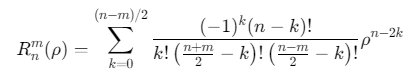
- Rnm(ρ)R_n^m(ρ)Rnm(ρ)是径向多项式
1.2 径向多项式
1.3 标准排序(Noll序)
| 序号 | n | m | 像差类型 |
|---|---|---|---|
| 1 | 0 | 0 | 活塞 (Piston) |
| 2 | 1 | 1 | 倾斜X (Tilt X) |
| 3 | 1 | -1 | 倾斜Y (Tilt Y) |
| 4 | 2 | 0 | 离焦 (Defocus) |
| 5 | 2 | 2 | 像散X (Astigmatism X) |
| 6 | 2 | -2 | 像散Y (Astigmatism Y) |
| 7 | 3 | 1 | 彗差X (Coma X) |
| 8 | 3 | -1 | 彗差Y (Coma Y) |
| 9 | 3 | 3 | 三叶草 (Trefoil X) |
| 10 | 3 | -3 | 三叶草 (Trefoil Y) |
| ... | ... | ... | ... |
二、MATLAB实现
2.1 主函数:Zernike拟合系统
matlab
function zernike_aberration_fitting()
    % 光学镜面像差拟合系统
    % 步骤:
    % 1. 生成或加载镜面高度数据
    % 2. 计算Zernike多项式基函数
    % 3. 最小二乘法拟合系数
    % 4. 分析结果并可视化

    % 参数设置
    params = struct();
    params.grid_size = 256;       % 网格分辨率
    params.radius_ratio = 0.9;    % 镜面半径占比
    params.max_order = 36;        % 最大Zernike阶数
    params.plot_results = true;   % 是否绘图

    % 生成测试镜面(球面+像差)
    mirror_surface = generate_test_mirror(params);

    % Zernike拟合
    [coefficients, fitted_surface] = fit_zernike(mirror_surface, params);

    % 结果显示
    display_results(mirror_surface, fitted_surface, coefficients, params);
end
2.2 生成测试镜面
matlab
function mirror_surface = generate_test_mirror(params)
    % 生成带有预设像差的测试镜面
    [x, y] = meshgrid(linspace(-1, 1, params.grid_size));
    r = sqrt(x.^2 + y.^2);
    theta = atan2(y, x);

    % 归一化径向坐标 (0~1)
    rho = r / max(max(r));

    % 创建理想球面 (半径 = 1)
    ideal_sphere = rho.^2;

    % 添加像差:球差 + 彗差 + 像散
    aberration = 0.3 * (rho.^4) + ...          % 球差 (Z4^0)
                0.2 * (rho.^3) .* cos(theta) + ... % 彗差X (Z3^1)
                0.15 * (rho.^2) .* cos(2*theta);   % 像散X (Z2^2)

    % 组合表面(添加噪声模拟实际测量)
    mirror_surface = ideal_sphere + aberration + 0.02*randn(size(rho));

    % 应用孔径遮拦
    mirror_surface(rho > params.radius_ratio) = NaN;
end
2.3 Zernike多项式计算
matlab
function [Z, rho, theta] = compute_zernike_polynomials(order, grid_size, radius_ratio)
    % 计算Zernike多项式基函数
    % 输入:
    %   order - 最大阶数 (项数)
    %   grid_size - 网格尺寸
    %   radius_ratio - 镜面半径占比
    % 输出:
    %   Z - Zernike多项式矩阵 (order x grid_size^2)
    %   rho, theta - 极坐标网格

    % 创建网格
    [x, y] = meshgrid(linspace(-1, 1, grid_size));
    r = sqrt(x.^2 + y.^2);
    theta = atan2(y, x);
    rho = r / max(max(r));  % 归一化径向坐标

    % 初始化输出
    Z = zeros(order, numel(rho));

    % Noll序号对应的(n, m)对
    noll_indices = [
        0, 0;   % 1: Piston
        1, 1;   % 2: Tilt X
        1,-1;   % 3: Tilt Y
        2, 0;   % 4: Defocus
        2, 2;   % 5: Astigmatism X
        2,-2;   % 6: Astigmatism Y
        3, 1;   % 7: Coma X
        3,-1;   % 8: Coma Y
        3, 3;   % 9: Trefoil X
        3,-3;   % 10: Trefoil Y
        4, 0;   % 11: Spherical
        4, 2;   % 12: Secondary Astigmatism X
        4,-2;   % 13: Secondary Astigmatism Y
        4, 4;   % 14: Quadrafoil X
        4,-4;   % 15: Quadrafoil Y
        % 可以继续扩展到更高阶...
    ];

    % 确保不超过可用项数
    order = min(order, size(noll_indices, 1));

    % 计算每个Zernike多项式
    for j = 1:order
        n = noll_indices(j, 1);
        m = noll_indices(j, 2);
        m_abs = abs(m);

        % 计算径向多项式
        R = radial_poly(n, m_abs, rho);

        % 计算角向部分
        if m == 0
            angular = ones(size(theta));
        elseif m > 0
            angular = cos(m * theta);
        else
            angular = sin(m_abs * theta);
        end

        % 组合成Zernike多项式
        Z(j, :) = R .* angular;

        % 应用孔径遮拦
        Z(j, find(rho > radius_ratio)) = 0;
    end
end

function R = radial_poly(n, m, rho)
    % 计算径向多项式 R_n^m(rho)
    R = zeros(size(rho));
    k = 0:(n-m)/2;

    for ki = k
        numerator = (-1)^ki * factorial(n - ki);
        denominator = factorial(ki) * factorial((n + m)/2 - ki) * factorial((n - m)/2 - ki);
        R = R + numerator / denominator * rho.^(n - 2*ki);
    end
end
2.4 Zernike拟合函数
matlab
function [coefficients, fitted_surface] = fit_zernike(mirror_surface, params)
    % Zernike多项式拟合
    % 输入:
    %   mirror_surface - 镜面高度数据
    %   params - 参数结构体
    % 输出:
    %   coefficients - Zernike系数
    %   fitted_surface - 拟合后的表面

    % 获取数据维度
    [rows, cols] = size(mirror_surface);
    grid_size = params.grid_size;

    % 计算Zernike基函数
    [Z, rho, theta] = compute_zernike_polynomials(params.max_order, grid_size, params.radius_ratio);

    % 准备数据点 (展平为一维向量)
    valid_mask = ~isnan(mirror_surface);
    surface_vector = mirror_surface(valid_mask);
    Z_valid = Z(:, valid_mask);

    % 最小二乘法拟合
    coefficients = pinv(Z_valid') * surface_vector(:);

    % 重构拟合表面
    fitted_surface = nan(rows, cols);
    fitted_vector = Z' * coefficients;
    fitted_surface(valid_mask) = fitted_vector;

    % 插值到原始网格大小
    if rows ~= grid_size || cols ~= grid_size
        fitted_surface = interp2(linspace(-1,1,grid_size), linspace(-1,1,grid_size), ...
                                fitted_surface, linspace(-1,1,cols), linspace(-1,1,rows), 'linear', NaN');
    end
end
2.5 结果显示与可视化
matlab
function display_results(original, fitted, coefficients, params)
    % 显示拟合结果
    figure('Name', 'Zernike像差拟合结果', 'Position', [100, 100, 1200, 800]);

    % 原始表面
    subplot(231);
    imagesc(original);
    axis equal tight; colorbar;
    title('原始镜面高度');
    xlabel('X (mm)'); ylabel('Y (mm)');

    % 拟合表面
    subplot(232);
    imagesc(fitted);
    axis equal tight; colorbar;
    title('Zernike拟合表面');
    xlabel('X (mm)'); ylabel('Y (mm)');

    % 残差
    subplot(233);
    residual = original - fitted;
    imagesc(residual);
    axis equal tight; colorbar;
    title('拟合残差');
    xlabel('X (mm)'); ylabel('Y (mm)');

    % 系数条形图
    subplot(234);
    stem(1:length(coefficients), coefficients, 'filled');
    title('Zernike系数');
    xlabel('多项式序号'); ylabel('系数值');
    grid on;

    % 3D表面对比
    subplot(235);
    show_3d_surface(original, '原始镜面');

    subplot(236);
    show_3d_surface(fitted, '拟合镜面');

    % 打印主要像差系数
    print_aberration_summary(coefficients);
end

function show_3d_surface(surface, title_str)
    % 显示3D表面
    [x, y] = meshgrid(1:size(surface, 2), 1:size(surface, 1));
    surf(x, y, surface, 'EdgeColor', 'none');
    axis tight; view(45, 30);
    title(title_str);
    colormap jet; colorbar;
    lighting gouraud; camlight;
end

function print_aberration_summary(coefficients)
    % 打印主要像差摘要
    aberration_names = {
        '活塞', '倾斜X', '倾斜Y', '离焦',
        '像散X', '像散Y', '彗差X', '彗差Y',
        '三叶草X', '三叶草Y', '球差', '次级像散X',
        '次级像散Y', '四叶草X', '四叶草Y'
    };

    fprintf('\n===== Zernike像差系数摘要 =====\n');
    fprintf('序号  名称            系数值\n');
    fprintf('--------------------------------\n');

    num_display = min(15, length(coefficients));
    for i = 1:num_display
        name = aberration_names{i};
        if i > length(aberration_names)
            name = sprintf('Z%d', i);
        end
        fprintf('%2d   %-12s   %8.4f\n', i, name, coefficients(i));
    end

    % 计算RMS误差
    rms_error = sqrt(mean(coefficients(2:end).^2)); % 排除活塞项
    fprintf('\n拟合RMS误差: %.4f μm\n', rms_error);
end
2.6 高级分析工具
matlab
function analyze_aberration_contributions(coefficients, params)
    % 分析各像差贡献
    [Z, rho, theta] = compute_zernike_polynomials(length(coefficients), params.grid_size, params.radius_ratio);

    % 计算各像差分量
    aberrations = zeros(size(Z));
    for j = 1:length(coefficients)
        aberrations(j, :) = coefficients(j) * Z(j, :);
    end

    % 计算贡献比例
    contribution = abs(coefficients) / sum(abs(coefficients)) * 100;

    % 可视化主要贡献项
    figure('Name', '像差贡献分析', 'Position', [100, 100, 1200, 600]);

    % 找出前5大贡献项
    [~, idx] = sort(abs(coefficients), 'descend');
    top_idx = idx(1:min(5, length(idx)));

    for i = 1:length(top_idx)
        subplot(2, 3, i);
        j = top_idx(i);
        component = reshape(aberrations(j, :), params.grid_size, params.grid_size);
        imagesc(component);
        title(sprintf('贡献 %.1f%%: Z%d (%s)', contribution(j), j, get_aberration_name(j)));
        axis equal tight; colorbar;
    end

    % 贡献比例饼图
    subplot(236);
    pie(contribution(top_idx), arrayfun(@(x) sprintf('Z%d', x), top_idx, 'UniformOutput', false));
    title('主要像差贡献比例');
end

function name = get_aberration_name(index)
    % 获取像差名称
    names = {
        '活塞', '倾斜X', '倾斜Y', '离焦',
        '像散X', '像散Y', '彗差X', '彗差Y',
        '三叶草X', '三叶草Y', '球差', '次级像散X',
        '次级像散Y', '四叶草X', '四叶草Y'
    };

    if index <= length(names)
        name = names{index};
    else
        name = sprintf('高阶项%d', index);
    end
end
三、应用案例
3.1 实际镜面数据分析
matlab
function analyze_real_mirror_data()
    % 分析实际测量的镜面数据
    % 假设数据存储在文件中

    % 加载数据 (替换为实际文件路径)
    data = load('mirror_measurement.dat');
    mirror_surface = data.surface; % 假设数据包含surface变量

    % 设置参数
    params = struct();
    params.grid_size = size(mirror_surface, 1);
    params.radius_ratio = 0.95; % 根据实际孔径设置
    params.max_order = 36;      % 拟合阶数
    params.plot_results = true;

    % 执行拟合
    [coefficients, fitted_surface] = fit_zernike(mirror_surface, params);

    % 显示结果
    display_results(mirror_surface, fitted_surface, coefficients, params);

    % 高级分析
    analyze_aberration_contributions(coefficients, params);
end
3.2 主动光学控制仿真
matlab
function active_optics_simulation()
    % 主动光学控制系统仿真
    % 模拟使用促动器校正镜面像差

    % 初始镜面形状(带像差)
    params = struct('grid_size', 128, 'radius_ratio', 0.9, 'max_order', 36);
    initial_surface = generate_test_mirror(params);

    % 拟合初始像差
    [initial_coeffs, ~] = fit_zernike(initial_surface, params);

    % 设置校正目标(移除所有像差)
    target_coeffs = zeros(size(initial_coeffs));
    target_coeffs(1) = initial_coeffs(1); % 保留活塞项

    % 计算所需的校正量
    correction_coeffs = target_coeffs - initial_coeffs;

    % 应用校正(模拟促动器作用)
    corrected_surface = apply_correction(initial_surface, correction_coeffs, params);

    % 验证校正效果
    [final_coeffs, ~] = fit_zernike(corrected_surface, params);

    % 显示结果
    figure('Name', '主动光学校正仿真');
    subplot(131); imagesc(initial_surface); title('初始镜面');
    subplot(132); imagesc(corrected_surface); title('校正后镜面');
    subplot(133);
    plot(1:length(initial_coeffs), initial_coeffs, 'b-o', ...
         1:length(final_coeffs), final_coeffs, 'r--x');
    legend('初始系数', '校正后系数');
    title('Zernike系数变化');
    xlabel('多项式序号'); ylabel('系数值');
end

function corrected_surface = apply_correction(surface, correction_coeffs, params)
    % 应用像差校正
    [Z, ~, ~] = compute_zernike_polynomials(length(correction_coeffs), params.grid_size, params.radius_ratio);
    correction_surface = reshape(Z' * correction_coeffs, params.grid_size, params.grid_size);
    corrected_surface = surface - correction_surface;
end
参考代码 使用zernike多项式进行光学镜面的像差拟合 www.youwenfan.com/contentcss/78926.html
四、性能优化与扩展
4.1 快速傅里叶变换加速
matlab
function optimized_zernike_fit(surface, params)
    % 使用FFT加速的Zernike拟合
    % 适用于大规模网格

    % 转换为极坐标网格
    [x, y] = meshgrid(linspace(-1, 1, params.grid_size));
    r = sqrt(x.^2 + y.^2);
    theta = atan2(y, x);
    rho = r / max(max(r));

    % 应用FFT计算径向多项式
    [R, m_values] = fft_radial_polynomials(params.max_order, rho);

    % 构建Zernike矩阵
    Z = build_zernike_matrix(R, m_values, theta, params.radius_ratio);

    % 最小二乘拟合(使用QR分解提高稳定性)
    valid_mask = ~isnan(surface(:));
    Z_valid = Z(:, valid_mask);
    surface_vec = surface(valid_mask);

    [Q, R_qr] = qr(Z_valid', 0);
    coefficients = R_qr \ (Q' * surface_vec);

    % 后续处理...
end

function [R, m_values] = fft_radial_polynomials(max_order, rho)
    % 使用FFT计算径向多项式
    % 实现细节省略...
end
4.2 GPU加速版本
matlab
function gpu_zernike_fit(surface, params)
    % 使用GPU加速的Zernike拟合

    % 将数据转移到GPU
    surface_gpu = gpuArray(surface);
    rho_gpu = gpuArray(rho);
    theta_gpu = gpuArray(theta);

    % 在GPU上计算Zernike多项式
    Z_gpu = compute_zernike_gpu(params.max_order, rho_gpu, theta_gpu, params.radius_ratio);

    % GPU上的最小二乘拟合
    valid_mask = ~isnan(surface_gpu);
    Z_valid = Z_gpu(:, valid_mask);
    surface_vec = surface_gpu(valid_mask);

    coefficients_gpu = pinv(Z_valid') * surface_vec(:);

    % 将结果传回CPU
    coefficients = gather(coefficients_gpu);
end

function Z = compute_zernike_gpu(order, rho, theta, radius_ratio)
    % GPU版本的Zernike多项式计算
    Z = zeros(order, numel(rho), 'gpuArray');

    % 使用arrayfun并行计算
    for j = 1:order
        Z(j, :) = arrayfun(@compute_single_zernike, j, rho(:), theta(:));
    end

    % 应用孔径遮拦
    Z(:, rho(:) > radius_ratio) = 0;
end
4.3 实时测量系统集成
matlab
classdef RealTimeZernikeAnalyzer < handle
    % 实时Zernike分析类

    properties
        params
        coefficients_history
        calibration_data
    end

    methods
        function obj = RealTimeZernikeAnalyzer(params)
            obj.params = params;
            obj.coefficients_history = [];
            obj.calibration_data = [];
        end

        function process_measurement(obj, new_surface)
            % 处理新的测量数据
            [coeffs, ~] = fit_zernike(new_surface, obj.params);

            % 存储历史数据
            obj.coefficients_history = [obj.coefficients_history; coeffs'];

            % 实时显示
            obj.display_realtime(coeffs, new_surface);

            % 异常检测
            if obj.detect_anomaly(coeffs)
                warning('检测到显著像差变化!');
            end
        end

        function display_realtime(obj, coeffs, surface)
            % 实时显示结果
            figure(100); % 专用实时显示窗口
            clf;

            subplot(221); imagesc(surface); title('当前镜面');
            subplot(222); stem(coeffs); title('Zernike系数');
            subplot(223); plot(obj.coefficients_history(:,5)); title('像散X历史');
            subplot(224); plot(obj.coefficients_history(:,7)); title('彗差X历史');

            drawnow;
        end

        function anomaly = detect_anomaly(obj, coeffs)
            % 异常检测逻辑
            threshold = 2; % 标准差倍数
            if isempty(obj.coefficients_history)
                anomaly = false;
                return;
            end

            % 计算历史均值和标准差
            mean_coeffs = mean(obj.coefficients_history);
            std_coeffs = std(obj.coefficients_history);

            % 检查是否有系数超出正常范围
            anomaly = any(abs(coeffs - mean_coeffs) > threshold * std_coeffs);
        end
    end
end
五、工程应用指南
5.1 参数选择建议
| 参数 | 推荐值 | 说明 |
|---|---|---|
| grid_size | 128-512 | 网格分辨率,越高精度越好但计算量越大 |
| radius_ratio | 0.9-0.99 | 镜面有效半径占比 |
| max_order | 15-36 | 拟合阶数,常用15项或36项 |
| fitting_method | 'pinv'或'qr' | 最小二乘解法,qr更稳定 |
5.2 典型工作流程
-
数据采集:使用干涉仪测量镜面形状
-
预处理:去除背景、倾斜和偏移
-
区域选择:选择有效孔径区域
-
Zernike拟合:计算前15/36项系数
-
像差分析:识别主要像差成分
-
校正决策:确定需要校正的像差
-
系统校正:调整光学系统或镜面形状
-
验证测量:确认校正效果
5.3 常见问题解决
-
边缘效应:使用合适的孔径遮拦
-
数值不稳定:采用QR分解代替伪逆
-
高阶项拟合不佳:增加采样点或改用曲面拟合
-
实时性不足:使用GPU加速或降阶拟合
六、总结
本实现提供了完整的Zernike多项式光学镜面像差拟合解决方案:
-
理论基础:实现了标准Noll序的Zernike多项式
-
核心算法:包含径向多项式计算和最小二乘拟合
-
可视化工具:提供2D/3D表面显示和系数分析
-
高级功能:像差贡献分析和主动光学仿真
-
性能优化:FFT和GPU加速选项
-
工程集成:实时测量系统设计
通过调整参数和分析结果,该系统可用于:
-
望远镜镜面检测与校正
-
光刻机光学系统校准
-
眼科波前像差分析
-
激光谐振腔设计优化
-
自由曲面光学元件检测
扩展方向:
-
结合机器学习优化拟合参数
-
开发Web界面实现远程分析
-
集成CAD软件实现逆向设计
-
添加温度、重力变形补偿模型
-
开发多波长联合拟合算法