matlab的高频注入

工具：Matlab2021a
电脑信息：Intel® Xeon® CPU E5-2603 v3 @ 1.60GHz
系统类型：64位操作系统，基于X64的处理器 windows10 专业版
通过千问获得代码：
cpp 复制代码
%% 高频注入 (HFI) 无位置传感器控制仿真示例
% 原理：脉振高频电压注入法 (Pulsating HFI)
% 适用：低速/零速下的 PMSM 转子位置估算
clear; clc; close all;

%% 1. 参数设置
fs = 20e3;              % 控制频率 (Hz)
Ts = 1/fs;              % 采样时间
T_sim = 0.5;            % 仿真总时间 (s)
t = 0:Ts:T_sim-Ts;      % 时间向量
N = length(t);

% 电机参数 (简化模型用)
Ld = 0.005;             % d轴电感 (H)
Lq = 0.008;             % q轴电感 (H) (假设 Lq > Ld，表贴式则相反或相等无法使用HFI)
Rs = 0.5;               % 电阻 (Ohm) - 高频下影响较小，此处忽略或简化
Pn = 4;                 % 极对数

% 高频注入参数
f_inj = 1000;           % 注入频率 (Hz)
w_inj = 2*pi*f_inj;     % 注入角频率
A_inj = 10;             % 注入电压幅值 (V)

% 真实转子运动 (模拟低速旋转)
w_real_rpm = 60;        % 真实转速 60 RPM
w_real_rad = w_real_rpm * 2*pi/60;
theta_real = cumsum(w_real_rad * Ts * ones(1, N)); % 真实位置累积

%% 2. 初始化变量
theta_est = 0;          % 估计位置初始值
w_est = 0;              % 估计速度
i_d_hf = zeros(1, N);   % 高频 d轴电流响应
i_q_hf = zeros(1, N);   % 高频 q轴电流响应
error_signal = zeros(1, N); % 位置误差信号
theta_est_vec = zeros(1, N); % 记录估计位置

% 滤波器参数 (简单的一阶低通滤波器用于解调后滤波)
fc_lpf = 200;           % 截止频率 Hz
alpha_lpf = 2*pi*fc_lpf*Ts / (1 + 2*pi*fc_lpf*Ts); 

filtered_error = 0;

% PLL 增益
Kp_pll = 500;           
Ki_pll = 10000;         
integrator_pll = 0;

%% 3. 主循环仿真
fprintf('开始仿真...\n');

for k = 1:N
    % --- 3.1 获取当前真实位置 ---
    th_true = theta_real(k);
    
    % --- 3.2 生成注入电压 (在估计的 d-q 坐标系下) ---
    % 我们在估计的 d 轴注入脉振电压: u_d_inj = A * sin(w_inj * t), u_q_inj = 0
    u_d_inj = A_inj * sin(w_inj * t(k));
    u_q_inj = 0;
    
    % --- 3.3 模拟电机高频响应 (基于磁路模型) ---
    % 坐标变换误差角度
    d_theta = th_true - theta_est;
    
    % 高频阻抗模型近似 (忽略电阻和反电势，仅考虑电感压降)
    % 实际物理量在真实 dq 轴，但我们在估计 dq 轴注入
    % 经过推导，响应电流中包含位置误差信息
    % 简化计算：直接计算在估计坐标系下的高频电流响应
    
    % 有效电感随位置误差变化
    % L_sigma = (Ld - Lq) / 2
    L_avg = (Ld + Lq) / 2;
    L_diff = (Ld - Lq) / 2;
    
    % 高频电流导数 di/dt = u / L_eff
    % 在估计坐标系下，由于电感矩阵的非对角项，q轴会产生高频电流
    % i_d_hf 主要受 Ld 影响 (近似)
    % i_q_hf 包含位置误差信息: i_q_hf ~ (Ld-Lq)/LdLq * sin(2*d_theta) * integral(u_d_inj)
    
    % 为了仿真效果，我们直接构造含有位置误差信息的响应电流
    % 真实物理过程是微分方程，这里用稳态近似加速仿真演示
    
    % d轴高频电流 (主要分量，与注入同相/滞后90度取决于模型，这里取积分关系)
    % u = L * di/dt => i = 1/L * integral(u)
    i_d_hf(k) = (1/Ld) * (-A_inj/w_inj) * cos(w_inj * t(k)); 
    
    % q轴高频电流 (包含位置误差的关键分量)
    % 幅度正比于 sin(2 * error_angle)
    amp_q = (Ld - Lq) / (Ld * Lq) * (A_inj / w_inj); 
    i_q_hf(k) = amp_q * sin(2 * d_theta) * cos(w_inj * t(k));
    
    % --- 3.4 信号解调 (Demodulation) ---
    % 将 q轴电流乘以注入信号的载波 (sin(w_inj * t))
    % 注意：相位匹配非常关键，这里假设理想匹配
    demod_raw = i_q_hf(k) * sin(w_inj * t(k));
    
    % --- 3.5 低通滤波 (LPF) ---
    % 提取直流分量，即位置误差信号
    filtered_error = filtered_error + alpha_lpf * (demod_raw - filtered_error);
    error_signal(k) = filtered_error;
    
    % --- 3.6 锁相环 (PLL) 更新估计位置 ---
    % 误差驱动 PLL
    % d_theta_est/dt = Kp * error + Ki * integral(error)
    prop_term = Kp_pll * error_signal(k);
    integrator_pll = integrator_pll + Ki_pll * error_signal(k) * Ts;
    
    w_est = prop_term + integrator_pll;
    theta_est = theta_est + w_est * Ts;
    
    % 限制角度在 -pi 到 pi
    theta_est = mod(theta_est + pi, 2*pi) - pi;
    
    theta_est_vec(k) = theta_est;
end

fprintf('仿真结束。\n');

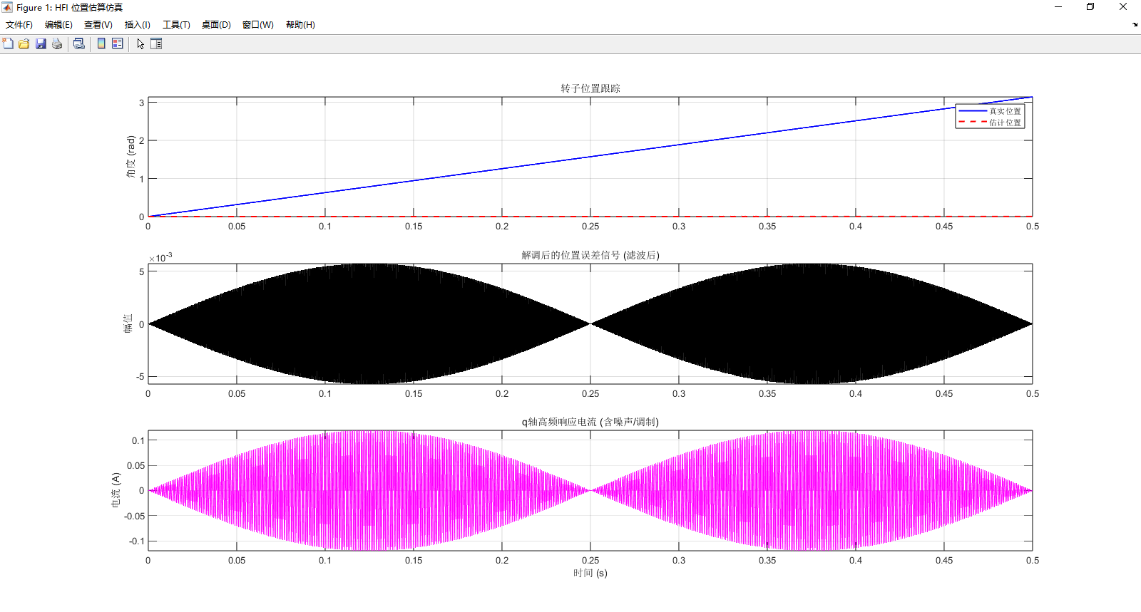
%% 4. 绘图结果
figure('Name', 'HFI 位置估算仿真', 'Color', 'w');

subplot(3,1,1);
plot(t, theta_real, 'b', 'LineWidth', 1.5); hold on;
plot(t, theta_est_vec, 'r--', 'LineWidth', 1.5);
legend('真实位置', '估计位置');
title('转子位置跟踪');
ylabel('角度 (rad)');
grid on;

subplot(3,1,2);
plot(t, error_signal, 'k', 'LineWidth', 1);
title('解调后的位置误差信号 (滤波后)');
ylabel('幅值');
grid on;

subplot(3,1,3);
plot(t, i_q_hf, 'm', 'LineWidth', 0.8);
title('q轴高频响应电流 (含噪声/调制)');
ylabel('电流 (A)');
xlabel('时间 (s)');
grid on;

% 误差分析
final_error = abs(theta_real(end) - theta_est_vec(end));
fprintf('最终位置误差: %.4f rad (%.2f 度)\n', final_error, rad2deg(final_error));
运行结果：