注:本文为 " PINN" 相关合辑。
图片清晰度受引文原图所限。
略作重排,未整理去重。
如有内容异常,请看原文。
偏微分方程的正问题和逆问题 (Inverse Problem)
Evavava 啊 原创于 2019-09-27 11:19:51
来源:《偏微分方程逆问题的数值方法及其应用》(苏超伟 1995)
该文献虽出版时间较早,但不影响对基础概念的理解。
(1)偏微分方程正问题


(2)偏微分方程逆问题

当偏微分方程中的微分算子、边界条件、初始条件由已知量变为未知量,且方程的解仍未确定时,此类问题即构成偏微分方程的逆(反)问题。

(3)研究方法与应用
在《DEEPXDE: A DEEP LEARNING LIBRARY FOR SOLVING DIFFERENTIAL EQUATIONS》中,提出采用物理信息神经网络(PINNs)求解偏微分方程逆问题的方法。

该方法认为,逆问题相较于正问题表现为未知参数数量增加,且具备更多可用于约束求解过程的已知条件。
PINN for PDE(偏微分方程)1 - 正向问题
小菜鸟博士 于 2025-06-01 20:41:57
一、PINN 正问题的定义
在 PINN(Physics-Informed Neural Networks,物理信息神经网络)中,正问题(Forward Problem) 定义为:
给定偏微分方程(PDE)的形式、边界条件与初始条件,求解该方程在定义域内的解函数。
在 PINN 框架下,求解正问题的基本步骤如下:
- 构建神经网络 u θ ( x , t ) u_\theta(x, t) uθ(x,t) 作为 PDE 解的近似;
- 利用自动微分计算偏导数,将 PDE 转化为损失函数项;
- 将边界条件和初始条件同样转化为损失函数;
- 通过最小化总损失训练神经网络参数 θ \theta θ,使其近似满足物理规律。
正问题的特征为:问题的数学描述是充分确定的,即 PDE 与条件信息足够完备,目标是通过神经网络模拟已知物理过程。
二、求解实例
待求解的偏微分方程如下:
∂ 2 u ∂ x 2 − ∂ 4 u ∂ y 4 = ( 2 − x 2 ) e − y \frac{\partial ^2u}{\partial x^2}-\frac{\partial ^4u}{\partial y^4}=\left( 2-x^2 \right) e^{-y} ∂x2∂2u−∂y4∂4u=(2−x2)e−y
2.1 边界条件
u y y ( x , 0 ) = x 2 u y y ( x , 1 ) = x 2 e u ( x , 0 ) = x 2 u ( x , 1 ) = x 2 e u ( 0 , y ) = 0 u ( 1 , y ) = e − y \begin{align*} u_{yy}\left( x,0 \right) &=x^2 \\ u_{yy}\left( x,1 \right) &=\frac{x^2}{e} \\ u\left( x,0 \right) &=x^2 \\ u\left( x,1 \right) &=\frac{x^2}{e} \\ u\left( 0,y \right) &=0 \\ u\left( 1,y \right) &=e^{-y} \end{align*} uyy(x,0)uyy(x,1)u(x,0)u(x,1)u(0,y)u(1,y)=x2=ex2=x2=ex2=0=e−y
2.2 解析解与定义域
该偏微分方程的解析解为:
u ( x , y ) = x 2 e − y u(x,y)=x^2 e^{-y} u(x,y)=x2e−y
其中, x x x 和 y y y 的取值范围均为 0 , 1 0,1 0,1。
三、基于 PyTorch 的实现代码
3.1 引入库函数
python
import torch
import matplotlib.pyplot as plt
from mpl_toolkits.mplot3d import Axes3D
3.2 设置超参数
python
# ====================== 超参数 ======================
epochs = 10000         # 训练轮数
h = 100                # 作图时的网格密度
N = 1000               # PDE 残差点(训练内点)
N1 = 100               # 边界条件点
N2 = 1000              # 数据点(已知解)
device = torch.device('cuda' if torch.cuda.is_available() else 'cpu')  # 设置计算设备
3.3 设置随机种子以保证结果可复现
python
def setup_seed(seed):
    torch.manual_seed(seed)  # 设置 CPU 随机数种子,保证 CPU 上随机数生成的可重复性
    torch.cuda.manual_seed_all(seed)  # 设置所有 GPU 设备的随机数种子
    torch.backends.cudnn.deterministic = True  # 强制 cuDNN 使用确定性算法,保证结果一致

# 设置随机数种子
setup_seed(888888)
cuDNN 确定性模式
cuDNN 为 NVIDIA 深度神经网络加速库,其通过自动选择最优卷积实现算法以提升计算效率。然而,部分优化算法采用非确定性计算策略(如浮点运算顺序差异),导致相同输入在不同执行中可能产生数值微小区别。
设置确定性模式将强制库仅使用确定性算法,消除计算顺序带来的随机性,确保前向传播与反向传播的数值结果完全可复现。该设置以牺牲部分计算性能为代价,换取实验的可重复性与调试的稳定性。
3.4 生成训练数据
python
"""
数据集构建模块:为偏微分方程(PDE)的物理信息神经网络(PINN)训练构建各类数据集,
涵盖区域内点、边界点的约束条件数据,以及解析解的真实数据,所有数据均包含坐标 (x, y) 和对应条件值。
"""
import torch

# 设备配置(示例,需根据实际环境定义)
device = torch.device("cuda" if torch.cuda.is_available() else "cpu")
# 采样点数配置(示例,需根据训练需求定义)
N, N1, N2 = 1000, 200, 500

# ===================== 偏微分方程约束条件数据生成 =====================
def interior(n=N):
    """
    生成 PDE 区域内点的训练数据(满足 PDE 微分约束)
    参数:
        n: 采样点数
    返回:
        x: 内点 x 坐标张量 (n,1),启用自动求导
        y: 内点 y 坐标张量 (n,1),启用自动求导
        cond: 内点对应的 PDE 约束真值,即 (2 - x²)·exp(-y)
    """
    x = torch.rand(n, 1).to(device)
    y = torch.rand(n, 1).to(device)
    cond = (2 - x ** 2) * torch.exp(-y)
    return x.requires_grad_(True), y.requires_grad_(True), cond

def down_yy(n=N1):
    """
    生成下边界(y=0)的二阶 y 偏导约束数据:u_yy(x, 0) = x²
    """
    x = torch.rand(n, 1).to(device)
    y = torch.zeros_like(x).to(device)
    cond = x ** 2
    return x.requires_grad_(True), y.requires_grad_(True), cond

def up_yy(n=N1):
    """
    生成上边界(y=1)的二阶 y 偏导约束数据:u_yy(x, 1) = x²/e
    """
    x = torch.rand(n, 1).to(device)
    y = torch.ones_like(x).to(device)
    cond = x ** 2 / torch.e
    return x.requires_grad_(True), y.requires_grad_(True), cond

def down(n=N1):
    """
    生成下边界(y=0)的函数值约束数据:u(x, 0) = x²
    """
    x = torch.rand(n, 1).to(device)
    y = torch.zeros_like(x).to(device)
    cond = x ** 2
    return x.requires_grad_(True), y.requires_grad_(True), cond

def up(n=N1):
    """
    生成上边界(y=1)的函数值约束数据:u(x, 1) = x²/e
    """
    x = torch.rand(n, 1).to(device)
    y = torch.ones_like(x).to(device)
    cond = x ** 2 / torch.e
    return x.requires_grad_(True), y.requires_grad_(True), cond

def left(n=N1):
    """
    生成左边界(x=0)的函数值约束数据:u(0, y) = 0
    """
    y = torch.rand(n, 1).to(device)
    x = torch.zeros_like(y).to(device)
    cond = torch.zeros_like(x)
    return x.requires_grad_(True), y.requires_grad_(True), cond

def right(n=N1):
    """
    生成右边界(x=1)的函数值约束数据:u(1, y) = exp(-y)
    """
    y = torch.rand(n, 1).to(device)
    x = torch.ones_like(y).to(device)
    cond = torch.exp(-y)
    return x.requires_grad_(True), y.requires_grad_(True), cond

# ===================== 解析解真实数据生成 =====================
def data_interior(n=N2):
    """
    生成 PDE 解析解的内点真实数据(用于监督学习)
    解析解为:u(x, y) = x²·exp(-y),据此生成坐标对应的真实函数值
    参数:
        n: 采样点数
    返回:
        x: 内点 x 坐标张量 (n,1),启用自动求导
        y: 内点 y 坐标张量 (n,1),启用自动求导
        cond: 解析解的真实函数值
    """
    x = torch.rand(n, 1).to(device)
    y = torch.rand(n, 1).to(device)
    cond = (x ** 2) * torch.exp(-y)
    return x.requires_grad_(True), y.requires_grad_(True), cond

"""
PINN 正向问题训练逻辑说明:
1. 数据构成:训练需两类数据------
   - 真实数据:由解析解生成的内点 (x, y) 及对应函数值,用于计算数据损失;
   - 边界约束数据:手动构建各边界的 (x, y) 及对应约束值(函数值/偏导值),用于计算边界损失。
2. 损失计算:
   - 将坐标信息输入网络得到预测值;
   - 内点预测值与真实数据对比,计算数据损失;
   - 边界点预测值与预设约束值对比,计算边界损失;
   - 综合两类损失优化网络,使模型满足 PDE 约束和边界条件。
"""
3.5 定义 PINN 网络结构
python
class MLP(torch.nn.Module):
    def __init__(self):
        super(MLP, self).__init__()
        self.net = torch.nn.Sequential(
            torch.nn.Linear(2, 32),
            torch.nn.Tanh(),
            torch.nn.Linear(32, 32),
            torch.nn.Tanh(),
            torch.nn.Linear(32, 32),
            torch.nn.Tanh(),
            torch.nn.Linear(32, 32),
            torch.nn.Tanh(),
            torch.nn.Linear(32, 1)
        )

    def forward(self, x):
        return self.net(x)

# 定义损失函数(均方误差)
loss_fn = torch.nn.MSELoss()
MSEloss, 其实就是平方损失,L2 距离
3.6 定义高阶导数计算函数
python
def gradients(u, x, order=1):
    """
    计算张量 u 对自变量 x 的指定阶数高阶导数(基于 PyTorch 自动求导实现)。

    参数:
        u (torch.Tensor): 待求导的函数输出张量(需与 x 维度匹配,且 x 需开启梯度追踪 requires_grad=True)。
        x (torch.Tensor): 自变量张量,作为求导的目标变量。
        order (int): 导数阶数,需为正整数,默认值为 1(一阶导数)。

    返回:
        torch.Tensor: u 对 x 的 order 阶导数张量,维度与输入 x 一致。

    实现说明:
        1. 基于 torch.autograd.grad 实现自动求导,通过嵌套调用支持高阶导数计算;
        2. grad 函数关键参数作用:
           - grad_outputs: 设为与 u 同形状的全1张量,用于将非标量输出 u 转换为标量(等价于对 u 所有元素求和后求导),保证非标量场景下求导有效;
           - create_graph: 设为 True,保留求导后的计算图,支持高阶导数的递归计算;
           - only_inputs: 设为 True,仅计算自变量 x 的梯度,排除其他无关张量的梯度计算;
        3. torch.autograd.grad 返回梯度元组(对应每个输入自变量的梯度),因仅对单个 x 求导,故取元组第一个元素作为结果。
    """
    if order == 1:
        # 计算一阶导数
        grad = torch.autograd.grad(
            outputs=u,
            inputs=x,
            grad_outputs=torch.ones_like(u),
            create_graph=True,
            only_inputs=True
        )
        return grad[0]
    else:
        # 递归嵌套计算高阶导数(n阶导数 = 对(n-1)阶导数再次求一阶导)
        return gradients(gradients(u, x, order=1), x, order=order - 1)
总结
- 该函数功能是基于 PyTorch 自动求导,通过递归嵌套实现张量 u 对自变量 x 的任意正整数阶导数计算;
create_graph=True是支持高阶导数的关键参数,grad_outputs=torch.ones_like(u)解决了非标量输出的求导适配问题;- 函数返回值为单一张量(取 grad 结果元组的第一个元素),维度与自变量 x 一致,保证使用便捷性。
函数返回一个元组,其中每个元素为对应输入张量的梯度。若inputs = [x, y],则返回 ( ∂ u / ∂ x , ∂ u / ∂ y ) (\partial u / \partial x, \partial u / \partial y) (∂u/∂x,∂u/∂y)。当仅有一个输入时,返回元组的第一个元素即可。
3.7 定义损失函数项
python
# PDE 残差损失
def l_interior(u):
    x, y, cond = interior()
    uxy = u(torch.cat([x, y], dim=1))
    return loss_fn(gradients(uxy, x, 2) - gradients(uxy, y, 4), cond)

# 边界损失:u_yy(x, 0) = x²
def l_down_yy(u):
    x, y, cond = down_yy()
    uxy = u(torch.cat([x, y], dim=1))
    return loss_fn(gradients(uxy, y, 2), cond)

# 边界损失:u_yy(x, 1) = x²/e
def l_up_yy(u):
    x, y, cond = up_yy()
    uxy = u(torch.cat([x, y], dim=1))
    return loss_fn(gradients(uxy, y, 2), cond)

# 边界损失:u(x, 0) = x²
def l_down(u):
    x, y, cond = down()
    uxy = u(torch.cat([x, y], dim=1))
    return loss_fn(uxy, cond)

# 边界损失:u(x, 1) = x²/e
def l_up(u):
    x, y, cond = up()
    uxy = u(torch.cat([x, y], dim=1))
    return loss_fn(uxy, cond)

# 边界损失:u(0, y) = 0
def l_left(u):
    x, y, cond = left()
    uxy = u(torch.cat([x, y], dim=1))
    return loss_fn(uxy, cond)

# 边界损失:u(1, y) = e^(-y)
def l_right(u):
    x, y, cond = right()
    uxy = u(torch.cat([x, y], dim=1))
    return loss_fn(uxy, cond)

# 解析解数据损失
def l_data(u):
    x, y, cond = data_interior()
    uxy = u(torch.cat([x, y], dim=1))
    return loss_fn(uxy, cond)
3.8 模型训练
python
# 初始化模型与优化器
u_model = MLP().to(device)
optimizer = torch.optim.Adam(params=u_model.parameters())

# 训练过程
for i in range(epochs):
    optimizer.zero_grad()  # 清除梯度
    # 计算总损失
    total_loss = l_interior(u_model) + l_up_yy(u_model) + l_down_yy(u_model) + \
                 l_up(u_model) + l_down(u_model) + l_left(u_model) + \
                 l_right(u_model) + l_data(u_model)
    total_loss.backward()  # 反向传播
    optimizer.step()       # 更新参数
    if i % 100 == 0:       # 每 100 轮打印进度
        print(f"Epoch {i}, Total Loss: {total_loss.item():.6f}")
3.9 结果可视化
python
# 推理与可视化
xc = torch.linspace(0, 1, h).to(device)
xm, ym = torch.meshgrid(xc, xc, indexing='ij')
xx = xm.reshape(-1, 1)
yy = ym.reshape(-1, 1)
xy = torch.cat([xx, yy], dim=1)
# 模型预测值与解析解
u_pred = u_model(xy)
u_real = xx * xx * torch.exp(-yy)
# 计算绝对误差
u_error = torch.abs(u_pred - u_real)
u_pred_fig = u_pred.reshape(h, h)
u_real_fig = u_real.reshape(h, h)
u_error_fig = u_error.reshape(h, h)
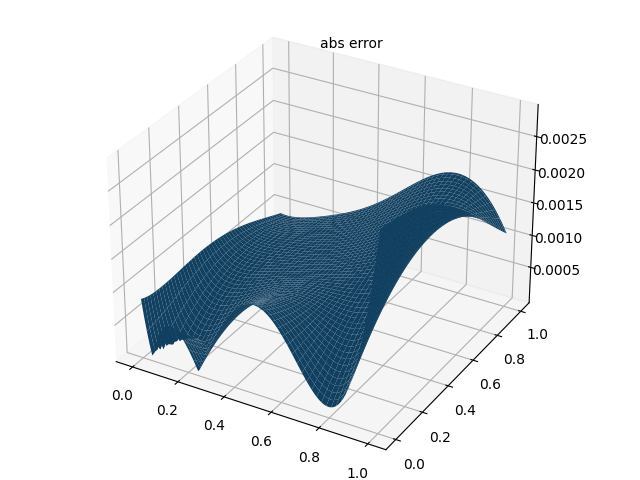
# 打印最大绝对误差
print("Max absolute error: ", float(torch.max(u_error)))
# 绘制 PINN 预测结果图
fig = plt.figure()
ax = Axes3D(fig)
fig.add_axes(ax)
ax.plot_surface(xm.cpu().detach().numpy(), ym.cpu().detach().numpy(),
u_pred_fig.cpu().detach().numpy(), cmap='viridis')
ax.set_xlabel('x')
ax.set_ylabel('y')
ax.set_zlabel('u')
ax.text2D(0.5, 0.9, "PINN Solution", transform=ax.transAxes, ha='center')
plt.savefig("PINN solve.png")
plt.show()
# 绘制解析解图
fig = plt.figure()
ax = Axes3D(fig)
fig.add_axes(ax)
ax.plot_surface(xm.cpu().detach().numpy(), ym.cpu().detach().numpy(),
u_real_fig.cpu().detach().numpy(), cmap='viridis')
ax.set_xlabel('x')
ax.set_ylabel('y')
ax.set_zlabel('u')
ax.text2D(0.5, 0.9, "Analytical Solution", transform=ax.transAxes, ha='center')
plt.savefig("real solve.png")
plt.show()
# 绘制误差图
fig = plt.figure()
ax = Axes3D(fig)
fig.add_axes(ax)
ax.plot_surface(xm.detach().cpu().numpy(), ym.cpu().detach().numpy(),
u_error_fig.cpu().detach().numpy(), cmap='Reds')
ax.set_xlabel('x')
ax.set_ylabel('y')
ax.set_zlabel('Absolute Error')
ax.text2D(0.5, 0.9, "Absolute Error", transform=ax.transAxes, ha='center')
plt.savefig("abs error.png")
plt.show()数值解验证与误差分析
验证流程
在求解域 Ω \Omega Ω 内随机采样空间坐标点 { ( x i , y i ) } i = 1 N \{(x_i, y_i)\}{i=1}^{N} {(xi,yi)}i=1N,通过解析解 u exact ( x , y ) u{\text{exact}}(x, y) uexact(x,y) 计算各点的精确场量值。将相同坐标输入训练完成的神经网络,获得预测数值解 u ^ ( x , y ) \hat{u}(x, y) u^(x,y)。逐点计算绝对误差:
ε i = ∣ u ^ ( x i , y i ) − u exact ( x i , y i ) ∣ \varepsilon_i = \left| \hat{u}(x_i, y_i) - u_{\text{exact}}(x_i, y_i) \right| εi=∣u^(xi,yi)−uexact(xi,yi)∣
或相对误差:
ε i rel = ∣ u ^ ( x i , y i ) − u exact ( x i , y i ) ∣ ∣ u exact ( x i , y i ) ∣ \varepsilon_i^{\text{rel}} = \frac{\left| \hat{u}(x_i, y_i) - u_{\text{exact}}(x_i, y_i) \right|}{\left| u_{\text{exact}}(x_i, y_i) \right|} εirel=∣uexact(xi,yi)∣∣u^(xi,yi)−uexact(xi,yi)∣
可视化结果
基于上述计算生成三组空间分布图:
- 精确解分布 : u exact ( x , y ) u_{\text{exact}}(x, y) uexact(x,y) 的真值云图
- 预测解分布 : u ^ ( x , y ) \hat{u}(x, y) u^(x,y) 的数值解云图
- 误差分布 : ε ( x , y ) \varepsilon(x, y) ε(x,y) 的逐点误差云图
四、结果展示
4.1 解析解结果图

4.2 PINN 预测结果图
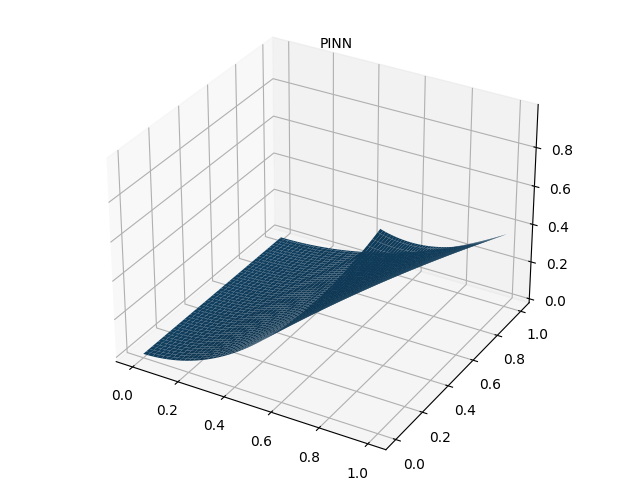
4.3 绝对误差图
五、参考文献
- PINN 解偏微分方程实例 1-CSDN 博客:https://blog.csdn.net/qq_49323609/article/details/129327571
- GitHub 仓库:https://github.com/YanxinTong/PINNs-for-PDE/tree/main/PINN_exp1_cs
PINN for PDE(偏微分方程)2 - 正向问题 - Diffusion
小菜鸟博士 于 2025-06-02 07:00:00
一、PINN 正问题的定义
在 PINN(Physics-Informed Neural Networks,物理信息神经网络)中,正问题(Forward Problem) 定义为:
给定偏微分方程(PDE)的形式、边界条件与初始条件,求解该方程在定义域内的解函数。
在 PINN 框架下,求解正问题的基本步骤如下:
- 构建神经网络 u θ ( x , t ) u_\theta(x, t) uθ(x,t) 作为 PDE 解的近似;
- 利用自动微分计算偏导数,将 PDE 转化为损失函数项;
- 将边界条件和初始条件同样转化为损失函数;
- 通过最小化总损失训练神经网络参数 θ \theta θ,使其近似满足物理规律。
正问题的特征为:问题的数学描述是充分确定的,即 PDE 与条件信息足够完备,目标是通过神经网络模拟已知物理过程。
二、扩散方程求解实例
2.1 扩散方程形式
一维扩散方程定义为:
∂ u ∂ t = ∂ 2 u ∂ x 2 + e − t ( − sin ( π x ) + π 2 sin ( π x ) ) , x ∈ − 1 , 1 , t ∈ 0 , 1 u ( x , 0 ) = sin ( π x ) u ( − 1 , t ) = u ( 1 , t ) = 0 \begin{align*} \frac{\partial u}{\partial t} &= \frac{\partial^2 u}{\partial x^2} + e^{-t} \left( -\sin(\pi x) + \pi^2 \sin(\pi x) \right), \quad x \in -1, 1, \ t \in 0, 1 \\ u(x, 0) &= \sin(\pi x) \\ u(-1, t) &= u(1, t) = 0 \end{align*} ∂t∂uu(x,0)u(−1,t)=∂x2∂2u+e−t(−sin(πx)+π2sin(πx)),x∈−1,1, t∈0,1=sin(πx)=u(1,t)=0
其中, u u u 表示扩散物质的浓度,该方程的解析解为:
u ( x , t ) = sin ( π x ) e − t u(x,t)=\sin(\pi x)e^{-t} u(x,t)=sin(πx)e−t
三、基于 PyTorch 的实现代码
3.1 引入库函数
python
import torch
import matplotlib.pyplot as plt
from mpl_toolkits.mplot3d import Axes3D
import os
3.2 设置超参数
python
# ====================== 超参数 ======================
epochs = 10000         # 训练轮数
h = 100                # 作图时的网格密度
N = 1000               # PDE 残差点(训练内点)
N1 = 100               # 边界条件点
N2 = 1000              # 数据点(已知解)
device = torch.device('cuda' if torch.cuda.is_available() else 'cpu')  # 设置计算设备
3.3 设置随机种子以保证结果可复现
python
def setup_seed(seed):
    torch.manual_seed(seed)  # 设置 CPU 随机数种子
    torch.cuda.manual_seed_all(seed)  # 设置所有 GPU 设备的随机数种子
    torch.backends.cudnn.deterministic = True  # 强制 cuDNN 使用确定性算法

# 设置随机数种子
setup_seed(888888)
cuDNN 是 NVIDIA 针对深度学习场景优化的加速库,为实现性能加速,该库在部分场景下会采用非确定性算法(例如执行卷积操作时,库会自动选择执行效率最优的实现方式,部分实现方式可能导致浮点运算的执行顺序存在差异)。
该配置可强制 cuDNN 仅调用确定性算法(此操作会牺牲一定的运算性能),从而确保前向传播与反向传播过程的计算结果在每次执行时均保持一致。
3.4 生成训练数据
python
"""
数据集构建模块:扩散方程(Diffusion Equation)物理信息神经网络(PINN)训练专用
==========================================================================
功能说明:
- 为PINN训练构建结构化数据集,输入为空间坐标x、时间坐标t,输出为函数值u
- 数据类型包含:内点约束数据、边界约束数据、解析解真实数据
- 所有张量默认部署在GPU(CUDA)上,无GPU时自动降级到CPU
"""
import torch

# ===================== 全局配置 =====================
# 设备配置:优先使用CUDA加速,否则使用CPU
device = torch.device("cuda" if torch.cuda.is_available() else "cpu")

# 采样点数配置(可根据训练需求调整)
N_INTERIOR = 1000    # 内点约束采样数
N_BOUNDARY = 200     # 边界约束采样数
N_ANALYTIC = 500     # 解析解真实数据采样数

# ===================== 偏微分方程约束条件数据生成 =====================
def generate_interior_points(n=N_INTERIOR):
    """
    生成扩散方程区域内点的训练数据(满足PDE微分约束)

    参数:
        n: 内点采样数量

    返回:
        x: 空间坐标张量 (n,1),范围 [-1,1),启用自动求导
        t: 时间坐标张量 (n,1),范围 [0,1),启用自动求导
        cond: 内点PDE约束真值
              计算公式:e^(-t) * (-sin(πx) + π²·sin(πx))
    """
    # 生成空间坐标:[0,1) → [-1,1)
    x = (torch.rand(n, 1) * 2 - 1).to(device)
    # 生成时间坐标:[0,1)
    t = torch.rand(n, 1).to(device)

    # 计算PDE约束真值
    sin_pi_x = torch.sin(torch.pi * x)
    cond = torch.exp(-t) * (-sin_pi_x + torch.pi**2 * sin_pi_x)

    return x.requires_grad_(True), t.requires_grad_(True), cond

def generate_initial_boundary(n=N_BOUNDARY):
    """
    生成初始边界(t=0)约束数据:u(x, 0) = sin(πx)

    参数:
        n: 边界点采样数量

    返回:
        x: 空间坐标张量 (n,1),范围 [-1,1),启用自动求导
        t: 时间坐标张量 (n,1),固定为 0,启用自动求导
        cond: 边界约束真值,即 sin(πx)
    """
    x = (torch.rand(n, 1) * 2 - 1).to(device)
    t = torch.zeros_like(x).to(device)
    cond = torch.sin(torch.pi * x)

    return x.requires_grad_(True), t.requires_grad_(True), cond

def generate_left_boundary(n=N_BOUNDARY):
    """
    生成左边界(x=-1)约束数据:u(-1, t) = 0

    参数:
        n: 边界点采样数量

    返回:
        x: 空间坐标张量 (n,1),固定为 -1,启用自动求导
        t: 时间坐标张量 (n,1),范围 [0,1),启用自动求导
        cond: 边界约束真值,固定为 0
    """
    t = torch.rand(n, 1).to(device)
    x = -torch.ones_like(t).to(device)
    cond = torch.zeros_like(t).to(device)

    return x.requires_grad_(True), t.requires_grad_(True), cond

def generate_right_boundary(n=N_BOUNDARY):
    """
    生成右边界(x=1)约束数据:u(1, t) = 0

    参数:
        n: 边界点采样数量

    返回:
        x: 空间坐标张量 (n,1),固定为 1,启用自动求导
        t: 时间坐标张量 (n,1),范围 [0,1),启用自动求导
        cond: 边界约束真值,固定为 0
    """
    t = torch.rand(n, 1).to(device)
    x = torch.ones_like(t).to(device)
    cond = torch.zeros_like(t).to(device)

    return x.requires_grad_(True), t.requires_grad_(True), cond

# ===================== 解析解真实数据生成 =====================
def generate_analytic_solution(n=N_ANALYTIC):
    """
    生成扩散方程解析解的内点真实数据(用于监督学习)

    解析解公式:u(x, t) = sin(πx) · e^(-t)

    参数:
        n: 真实数据采样数量

    返回:
        x: 空间坐标张量 (n,1),范围 [-1,1),启用自动求导
        t: 时间坐标张量 (n,1),范围 [0,1),启用自动求导
        cond: 解析解真实值,即 sin(πx) · e^(-t)
    """
    x = (torch.rand(n, 1) * 2 - 1).to(device)
    t = torch.rand(n, 1).to(device)
    cond = torch.sin(torch.pi * x) * torch.exp(-t)

    return x.requires_grad_(True), t.requires_grad_(True), cond

"""
PINN 正向问题训练逻辑说明
========================
1. 数据构成:
   - 真实数据:由解析解生成的内点 (x, t) 及对应函数值,用于计算数据损失
   - 边界约束数据:手动构建各边界的 (x, t) 及对应约束值,用于计算边界损失

2. 损失计算:
   - 将坐标信息 (x, t) 输入网络得到预测值 û
   - 内点预测值与真实数据对比,计算数据损失(监督损失)
   - 边界点预测值与预设约束值对比,计算边界损失(物理约束损失)
   - 综合两类损失优化网络,使模型满足扩散方程约束和边界条件
"""- 数据集构建覆盖内点(
interior)、三类边界点(down_1/down_2/down_3)及真实观测数据(data_interior),均返回带自动求导的x/t与对应真值项; - PINN 正向问题数据为真实观测数据与边界条件数据,格式均为
(坐标输入, 目标值); - 训练时需区分内点/边界点分别计算损失,边界损失单独计算是为保证模型满足预设边界约束。
3.5 定义 PINN 网络结构
python
class MLP(torch.nn.Module):
    def __init__(self):
        super(MLP, self).__init__()
        self.net = torch.nn.Sequential(
            torch.nn.Linear(2, 32),
            torch.nn.Tanh(),
            torch.nn.Linear(32, 32),
            torch.nn.Tanh(),
            torch.nn.Linear(32, 32),
            torch.nn.Tanh(),
            torch.nn.Linear(32, 32),
            torch.nn.Tanh(),
            torch.nn.Linear(32, 1)
        )

    def forward(self, x):
        return self.net(x)

# 定义损失函数(均方误差)
loss_fn = torch.nn.MSELoss()
3.6 定义高阶导数计算函数
python
def gradients(u, x, order=1):
    """
    计算函数 u 对变量 x 的高阶导数(PINN 工具函数)

    用途说明:
    - 用于物理信息神经网络 (PINN) 中计算 PDE 的微分约束
    - 支持任意阶数的导数计算,基于 PyTorch 自动求导实现
    - 仅用于求导计算,不会修改输入张量的内容

    参数:
        u (torch.Tensor): 待求导的函数输出张量(需与 x 维度匹配)
        x (torch.Tensor): 自变量张量(必须启用 requires_grad=True)
        order (int): 导数的阶数,默认为 1(一阶导数)

    返回:
        torch.Tensor: u 对 x 的指定阶数导数,维度与输入保持一致

    示例:
        >>> x = torch.tensor([1.0, 2.0], requires_grad=True)
        >>> u = x**2
        >>> gradients(u, x)  # 一阶导数:2x
        tensor([2., 4.])
        >>> gradients(u, x, order=2)  # 二阶导数:2
        tensor([2., 2.])
    """
    # ========== torch.autograd.grad 参数详解 ==========
    # u (outputs): 待求导的目标张量(标量/向量)
    # x (inputs): 求导的自变量(需 requires_grad=True)
    # grad_outputs: 非标量输出时的梯度权重(全 1 表示直接求和)
    # create_graph: 保留计算图,支持高阶导数(必须设为 True)
    # only_inputs: 仅计算 inputs 的梯度,忽略其他中间变量

    # 一阶导数计算
    if order == 1:
        return torch.autograd.grad(
            outputs=u,
            inputs=x,
            grad_outputs=torch.ones_like(u),
            create_graph=True,
            only_inputs=True
        )[0]

    # 高阶导数:递归嵌套求导
    else:
        # 阶数校验,避免无效递归
        if not isinstance(order, int) or order < 1:
            raise ValueError(f"导数阶数必须为正整数,当前输入:{order}")
return gradients(gradients(u, x), x, order=order - 1)- 函数
gradients专注于求导功能,仅计算导数不修改输入变量,当前版本仅实现一阶导数计算; torch.autograd.grad是求导接口,create_graph=True是高阶导数计算的关键,grad_outputs用于非标量输出的梯度合成;- 函数返回值为元组的第一个元素,因仅对单个自变量 x 求导,直接取该元素即可得到对应导数张量。
3.7 定义损失函数项
python
# PDE 残差损失
def l_interior(u):
    x, t, cond = interior()
    uxt = u(torch.cat([x, t], dim=1))
    return loss_fn(gradients(uxt, t, 1) - gradients(uxt, x, 2), cond)

# 初始条件损失:u(x, 0) = sin(πx)
def l_down_1(u):
    x, t, cond = down_1()
    uxt = u(torch.cat([x, t], dim=1))
    return loss_fn(uxt, cond)

# 边界损失:u(-1, t) = 0
def l_down_2(u):
    x, t, cond = down_2()
    uxt = u(torch.cat([x, t], dim=1))
    return loss_fn(uxt, cond)

# 边界损失:u(1, t) = 0
def l_down_3(u):
    x, t, cond = down_3()
    uxt = u(torch.cat([x, t], dim=1))
    return loss_fn(uxt, cond)

# 解析解数据损失
def l_data(u):
    x, t, cond = data_interior()
    uxt = u(torch.cat([x, t], dim=1))
    return loss_fn(uxt, cond)
3.8 模型训练
python
# 初始化模型与优化器
u_model = MLP().to(device)
optimizer = torch.optim.Adam(params=u_model.parameters())

# 训练过程
for i in range(epochs):
    optimizer.zero_grad()  # 清除梯度
    # 计算总损失
    total_loss = l_interior(u_model) + l_down_1(u_model) + l_down_2(u_model) + \
                 l_down_3(u_model) + l_data(u_model)
    total_loss.backward()  # 反向传播
    optimizer.step()       # 更新参数
    if i % 100 == 0:       # 每 100 轮打印进度
        print(f"Epoch {i}, Total Loss: {total_loss.item():.6f}")
3.9 结果可视化
python
"""
推理模块:扩散方程 PINN 模型预测结果验证
========================================
功能说明:
- 在指定空间和时间范围内采样,计算模型预测值与解析解真实值
- 对比预测值与真实值的绝对误差,输出最大误差值
- 绘制 3D 可视化图:PINN 数值解、解析解真实值、绝对误差分布
"""
import os
import torch
import matplotlib.pyplot as plt
from mpl_toolkits.mplot3d import Axes3D

# ===================== 推理参数配置 =====================
# 网格采样点数(可根据可视化精度调整)
h = 100  # x 和 t 方向的采样数量一致
# 设备配置(与训练保持一致)
device = torch.device("cuda" if torch.cuda.is_available() else "cpu")

# ===================== 数据准备与预测 =====================
# 生成空间和时间网格:x 范围 (-1,1),t 范围 (0,1)
xc = torch.linspace(-1, 1, h).to(device)
tc = torch.linspace(0, 1, h).to(device)
xm, tm = torch.meshgrid(xc, tc, indexing='ij')  # 生成网格坐标

# 转换为模型输入格式 (n, 2):n = h * h
xx = xm.reshape(-1, 1)  # 空间坐标展平
tt = tm.reshape(-1, 1)  # 时间坐标展平
xt = torch.cat([xx, tt], dim=1)  # 拼接为 [x, t] 输入

# 模型预测与真实值计算
u_pred = u(xt)  # PINN 模型预测值(需确保 u 是已训练好的模型)
u_real = torch.sin(torch.pi * xx) * torch.exp(-tt)  # 解析解真实值:sin(πx)·exp(-t)

# ===================== 误差计算 =====================
u_error = torch.abs(u_pred - u_real)  # 逐点绝对误差
max_abs_error = float(torch.max(u_error))  # 最大绝对误差

# 重塑为网格格式用于绘图 (h, h)
u_pred_fig = u_pred.reshape(h, h)
u_real_fig = u_real.reshape(h, h)
u_error_fig = u_error.reshape(h, h)

# 输出误差信息
print("Max abs error is: ", max_abs_error)
# 参考结果:
# - 仅有 PDE 损失: 0.004852950572967529
# - 带有数据点损失: 0.0018916130065917969

# ===================== 结果可视化与保存 =====================
# 创建结果保存目录(不存在则创建)
os.makedirs("result_img", exist_ok=True)

# 辅助函数:简化 3D 绘图流程
def plot_3d_surface(x, y, z, title, save_path):
    """
    绘制 3D 曲面图并保存

    参数:
        x (torch.Tensor): x 轴数据(网格)
        y (torch.Tensor): y 轴数据(网格)
        z (torch.Tensor): z 轴数据(网格)
        title (str): 图表标题
        save_path (str): 保存路径
    """
    # 转换为 numpy 数组(CPU 上计算)
    x_np = x.cpu().detach().numpy()
    y_np = y.cpu().detach().numpy()
    z_np = z.cpu().detach().numpy()

    # 创建 3D 绘图
    fig = plt.figure(figsize=(8, 6))
    ax = Axes3D(fig)
    fig.add_axes(ax)

    # 绘制曲面
    ax.plot_surface(x_np, y_np, z_np, cmap='viridis')
    ax.set_xlabel('x')
    ax.set_ylabel('t')
    ax.set_zlabel('u')
    ax.text2D(0.5, 0.9, title, transform=ax.transAxes, ha='center')

    # 显示并保存
    plt.tight_layout()
    plt.show()
    fig.savefig(save_path, dpi=300, bbox_inches='tight')
    plt.close(fig)

# 1. 绘制 PINN 数值解图
plot_3d_surface(xm, tm, u_pred_fig, "PINN solve", "result_img/PINN solve.png")

# 2. 绘制解析解真实值图
plot_3d_surface(xm, tm, u_real_fig, "real solve", "result_img/real solve.png")

# 3. 绘制绝对误差图
plot_3d_surface(xm, tm, u_error_fig, "abs error", "result_img/abs error.png")
四、结果展示
4.1 解析解结果图
4.2 PINN 预测结果图
4.3 绝对误差图

五、参考文献
- PINN 解偏微分方程实例 4--Diffusion,Burgers,Allen--Cahn 和 Wave 方程和反问题代码:https://blog.csdn.net/qq_49323609/article/details/139906996
- GitHub 仓库:https://github.com/YanxinTong/PINNs-for-PDE/tree/main/PINN_exp2_Diffusion
PINN for PDE(偏微分方程)3 - 正向问题 - Burgers' equation
小菜鸟博士 于 2025-06-02 08:00:00
一、PINN 正问题的定义
在 PINN(Physics-Informed Neural Networks,物理信息神经网络)中,正问题(Forward Problem) 定义为:
给定偏微分方程(PDE)的形式、边界条件与初始条件,求解该方程在定义域内的解函数。
在 PINN 框架下,求解正问题的基本步骤如下:
- 构建神经网络 u θ ( x , t ) u_\theta(x, t) uθ(x,t) 作为 PDE 解的近似;
- 利用自动微分计算偏导数,将 PDE 转化为损失函数项;
- 将边界条件和初始条件同样转化为损失函数;
- 通过最小化总损失训练神经网络参数 θ \theta θ,使其近似满足物理规律。
正问题的特征为:问题的数学描述是充分确定的,即 PDE 与条件信息足够完备,目标是通过神经网络模拟已知物理过程。
二、Burgers 方程求解实例
2.1 Burgers 方程形式
Burgers 方程定义为:
∂ u ∂ t + u ∂ u ∂ x = ν ∂ 2 u ∂ x 2 , x ∈ − 1 , 1 , t ∈ 0 , 1 u ( x , 0 ) = − sin ( π x ) u ( − 1 , t ) = u ( 1 , t ) = 0 \begin{align*} \frac{\partial u}{\partial t} + u \frac{\partial u}{\partial x} &= \nu \frac{\partial^2 u}{\partial x^2}, \quad x \in -1, 1, \ t \in 0, 1 \\ u(x, 0) &= -\sin(\pi x) \\ u(-1, t) &= u(1, t) = 0 \end{align*} ∂t∂u+u∂x∂uu(x,0)u(−1,t)=ν∂x2∂2u,x∈−1,1, t∈0,1=−sin(πx)=u(1,t)=0
其中, u u u 表示流速, ν \nu ν 为流体粘度,本文中设置 ν = 0.01 / π \nu = 0.01 / \pi ν=0.01/π。
2.2 数值解法:线方法结合四阶龙格-库塔法(MOL-RK4)
由于 Burgers 方程无显式解析解,采用线方法(Method of Lines, MOL) 结合四阶龙格-库塔法(RK4)求解其数值解,作为 PINN 训练的参考数据。具体步骤为:首先利用有限差分法(或谱方法)对空间导数进行离散,将偏微分方程转化为关于时间的常微分方程组;随后采用 RK4 方法进行时间积分。RK4 是求解常微分方程初值问题(IVP)的经典显式方法,具有四阶精度,局部截断误差为 O ( Δ t 5 ) O(\Delta t^5) O(Δt5),全局误差为 O ( Δ t 4 ) O(\Delta t^4) O(Δt4),其中 Δ t \Delta t Δt 为时间步长。
2.2.1 RK4 基本公式
对于常微分方程 d y d t = f ( t , y ) \frac{\mathrm{d}\boldsymbol{y}}{\mathrm{d}t} = \boldsymbol{f}(t, \boldsymbol{y}) dtdy=f(t,y),初始条件 y ( t 0 ) = y 0 \boldsymbol{y}(t_0) = \boldsymbol{y}_0 y(t0)=y0,RK4 的迭代格式为:
k 1 = f ( t n , y n ) k 2 = f ( t n + Δ t 2 , y n + Δ t 2 k 1 ) k 3 = f ( t n + Δ t 2 , y n + Δ t 2 k 2 ) k 4 = f ( t n + Δ t , y n + Δ t k 3 ) y n + 1 = y n + Δ t 6 ( k 1 + 2 k 2 + 2 k 3 + k 4 ) \begin{aligned} \boldsymbol{k}_1 &= \boldsymbol{f}\!\left(t_n, \boldsymbol{y}_n\right) \\ \boldsymbol{k}_2 &= \boldsymbol{f}\!\left(t_n + \frac{\Delta t}{2}, \boldsymbol{y}_n + \frac{\Delta t}{2}\boldsymbol{k}_1\right) \\ \boldsymbol{k}_3 &= \boldsymbol{f}\!\left(t_n + \frac{\Delta t}{2}, \boldsymbol{y}_n + \frac{\Delta t}{2}\boldsymbol{k}_2\right) \\ \boldsymbol{k}_4 &= \boldsymbol{f}\!\left(t_n + \Delta t, \boldsymbol{y}_n + \Delta t\,\boldsymbol{k}3\right) \\ \boldsymbol{y}{n+1} &= \boldsymbol{y}_n + \frac{\Delta t}{6}\left(\boldsymbol{k}_1 + 2\boldsymbol{k}_2 + 2\boldsymbol{k}_3 + \boldsymbol{k}_4\right) \end{aligned} k1k2k3k4yn+1=f(tn,yn)=f(tn+2Δt,yn+2Δtk1)=f(tn+2Δt,yn+2Δtk2)=f(tn+Δt,yn+Δtk3)=yn+6Δt(k1+2k2+2k3+k4)
其中, Δ t \Delta t Δt 为时间步长, t n + 1 = t n + Δ t t_{n+1} = t_n + \Delta t tn+1=tn+Δt。在 MOL 框架下, y \boldsymbol{y} y 为空间离散点上的解向量, f \boldsymbol{f} f 包含空间离散后的残差项。
2.2.2 常用时间积分方法对比
| 方法 | 局部截断误差 | 全局误差 | 显/隐式 | 稳定性 | 适用场景 |
|---|---|---|---|---|---|
| 前向欧拉法 | O ( Δ t 2 ) O(\Delta t^2) O(Δt2) | O ( Δ t ) O(\Delta t) O(Δt) | 显式 | 条件稳定 | 简单实现,教学演示 |
| 二阶龙格-库塔(中点法) | O ( Δ t 3 ) O(\Delta t^3) O(Δt3) | O ( Δ t 2 ) O(\Delta t^2) O(Δt2) | 显式 | 条件稳定 | 精度要求中等 |
| 四阶龙格-库塔(RK4) | O ( Δ t 5 ) O(\Delta t^5) O(Δt5) | O ( Δ t 4 ) O(\Delta t^4) O(Δt4) | 显式 | 条件稳定 | 精度与效率兼顾(本文采用) |
| 后向欧拉法 | O ( Δ t 2 ) O(\Delta t^2) O(Δt2) | O ( Δ t ) O(\Delta t) O(Δt) | 隐式 | 无条件稳定 | 刚性问题 |
| 隐式 RK(如 Radau、Gauss) | O ( Δ t p + 1 ) O(\Delta t^{p+1}) O(Δtp+1) | O ( Δ t p ) O(\Delta t^p) O(Δtp) | 隐式 | 无条件稳定 | 高精度刚性问题 |
三、基于 PyTorch 的实现代码
3.1 longge.py(RK4 求解 Burgers 方程)
python
""" Solving the Burgers' Equation using 4th order Runge-Kutta (RK4) method
核心改进:
1. 修复绘图顺序,先保存后显示
2. 统一变量命名,增加参数校验
3. 补充异常处理,增强鲁棒性
"""
import numpy as np
import matplotlib.pyplot as plt
from mpl_toolkits.mplot3d import Axes3D
from matplotlib import cm
import os

def rk4(f, u, t, dx, h):
    """四阶龙格-库塔法计算下一时间步的u值
    参数:
        f: 右端项函数
        u: 当前时间步的u值数组
        t: 当前时间
        dx: 空间步长
        h: RK4时间步长
    返回:
        下一时间步的u值
    """
    k1 = f(u, t, dx)
    k2 = f(u + 0.5*h*k1, t + 0.5*h, dx)
    k3 = f(u + 0.5*h*k2, t + 0.5*h, dx)
    k4 = f(u + h*k3, t + h, dx)
    return u + (h/6)*(k1 + 2*k2 + 2*k3 + k4)

def dudx(u, dx):
    """中心差分法计算一阶导数(周期边界)"""
    first_deriv = np.zeros_like(u)
    first_deriv[0] = (u[1] - u[-1]) / (2*dx)
    first_deriv[-1] = (u[0] - u[-2]) / (2*dx)
    first_deriv[1:-1] = (u[2:] - u[0:-2]) / (2*dx)
    return first_deriv

def d2udx2(u, dx):
    """中心差分法计算二阶导数(周期边界)"""
    second_deriv = np.zeros_like(u)
    second_deriv[0] = (u[1] - 2*u[0] + u[-1]) / (dx**2)
    second_deriv[-1] = (u[0] - 2*u[-1] + u[-2]) / (dx**2)
    second_deriv[1:-1] = (u[2:] - 2*u[1:-1] + u[0:-2]) / (dx**2)
    return second_deriv

def f(u, t, dx, nu=0.01/np.pi):
    """Burgers方程右端项:∂u/∂t = -u∂u/∂x + ν∂²u/∂x²"""
    return -u*dudx(u, dx) + nu*d2udx2(u, dx)

def burgers(x0, xN, N, t0, tK, K):
    """求解Burgers方程
    参数:
        x0,xN: 空间范围
        N: 空间网格数
        t0,tK: 时间范围
        K: 时间步数
    返回:
        X,T: 空间-时间网格
        u: 数值解数组 (K, N)
    """
    # 参数校验
    if N < 3:
        raise ValueError("空间网格数N必须≥3(保证中心差分有效)")
    if K < 2:
        raise ValueError("时间步数K必须≥2")

    x = np.linspace(x0, xN, N)
    dx = (xN - x0) / (N - 1)
    dt = (tK - t0) / (K - 1)  # 修正:原代码用K,应改为K-1(网格数=步数+1)
    h = 2e-6  # RK4小步长

    u = np.zeros((K, N))
    u[0, :] = -np.sin(np.pi*x)  # 初始条件

    # 时间迭代
    for idx in range(K-1):
        ti = t0 + dt*idx
        U = u[idx, :]
        # RK4迭代到下一个时间步
        for step in range(1000):
            t = ti + h*step
            U = rk4(f, U, t, dx, h)
        u[idx+1, :] = U

    X, T = np.meshgrid(x, np.linspace(t0, tK, K))
    return X, T, u

# 求解参数
x0, xN, N = -1, 1, 512
t0, tK, K = 0, 1, 500

# 创建保存目录
os.makedirs("result_img", exist_ok=True)

# 求解方程
X, T, u = burgers(x0, xN, N, t0, tK, K)

if __name__ == '__main__':
    # 绘制3D曲面图
    fig = plt.figure(figsize=(10, 6))
    ax = fig.add_subplot(111, projection='3d')
    surf = ax.plot_surface(X, T, u, cmap=cm.viridis, linewidth=0, antialiased=True)
    ax.set_xlabel('x')
    ax.set_ylabel('t')
    ax.set_zlabel('u')
    ax.set_title("Burgers Equation (RK4 Solution)")
    fig.colorbar(surf, shrink=0.5, aspect=5)

    # 先保存后显示(关键!)
    plt.savefig("result_img/burgers.png", dpi=300, bbox_inches='tight')
    plt.show()
3.2 main.py(PINN 求解 Burgers 方程)
3.2.1 引入库函数
python
import torch
import matplotlib.pyplot as plt
from mpl_toolkits.mplot3d import Axes3D
import os
from longge import X, T, Z  # 导入 RK4 求解的数值解
3.2.2 设置超参数
python
# ====================== 超参数 ======================
epochs = 10000         # 训练轮数
h = 100                # 作图时的网格密度
N = 1000               # PDE 残差点(训练内点)
N1 = 100               # 边界条件点
N2 = 1000              # 数据点(已知解)
device = torch.device('cuda' if torch.cuda.is_available() else 'cpu')  # 设置计算设备
3.2.3 设置随机种子以保证结果可复现
python
import torch

def setup_seed(seed):
    """
    配置随机数种子,保障实验结果可复现
    参数:
        seed (int): 随机数种子数值
    """
    torch.manual_seed(seed)  # 配置 PyTorch 框架下 CPU 端随机数种子,使 torch.rand()、torch.randn() 等函数在 CPU 端生成的随机数具备可重复性
    torch.cuda.manual_seed_all(seed)  # 配置全部 GPU 设备的随机数种子,GPU 独立随机数生成器应用于模型参数初始化、Dropout 等操作
    torch.backends.cudnn.deterministic = True  # 强制 cuDNN 库仅调用确定性算法(以少量运算效率为代价),规避非确定性算法引发的计算结果偏差
    # 可选配置:关闭 cuDNN 基准模式,进一步保障确定性(若追求运算效率可注释该行)
    # torch.backends.cudnn.benchmark = False

# 执行随机数种子配置
setup_seed(888888)
3.2.4 生成训练数据
python
import torch

# 定义计算设备(需提前初始化 device 变量,如 device = torch.device("cuda" if torch.cuda.is_available() else "cpu"))
# device = torch.device("cuda" if torch.cuda.is_available() else "cpu")

# Domain and Sampling:Burgers 方程输入为 x、t,输出为 u
def interior(n=N):
    """
    生成偏微分方程(PDE)求解区域内点的训练样本
    参数:
        n (int): 生成样本数量,默认值为 N
    返回:
        x (torch.Tensor): 形状为 (n, 1) 的 x 坐标张量,范围 [-1, 1),启用自动求导
        t (torch.Tensor): 形状为 (n, 1) 的 t 坐标张量,范围 [0, 1),启用自动求导
        cond (torch.Tensor): 形状为 (n, 1) 的条件值张量,取值为 0
    """
    # 生成 [-1, 1) 范围内的 x 坐标:将 torch.rand() 生成的 [0,1) 均匀分布数据线性变换至目标区间
    x = (torch.rand(n, 1) * 2 - 1).to(device)
    # 生成 [0, 1) 范围内的 t 坐标
    t = torch.rand(n, 1).to(device)
    # 初始化条件值张量(与 t 形状一致,取值为 0),用于损失函数计算
    cond = torch.zeros_like(t).to(device)

    return x.requires_grad_(True), t.requires_grad_(True), cond

def down_1(n=N1):
    """
    生成 Burgers 方程下边界(t=0)的训练样本,满足边界条件 u(x, 0) = -sin(πx)
    参数:
        n (int): 生成样本数量,默认值为 N1
    返回:
        x (torch.Tensor): 形状为 (n, 1) 的 x 坐标张量,范围 [-1, 1),启用自动求导
        t (torch.Tensor): 形状为 (n, 1) 的 t 坐标张量,取值为 0,启用自动求导
        cond (torch.Tensor): 形状为 (n, 1) 的边界条件值张量,取值为 -sin(πx)
    """
    # 生成 [-1, 1) 范围内的 x 坐标
    x = (torch.rand(n, 1) * 2 - 1).to(device)
    # 初始化 t 坐标张量(与 x 形状一致,取值为 0)
    t = torch.zeros_like(x).to(device)
    # 计算边界条件值:u(x, 0) = -sin(πx)
    cond = -torch.sin(torch.pi * x)

    return x.requires_grad_(True), t.requires_grad_(True), cond

def down_2(n=N1):
    """
    生成 Burgers 方程左边界(x=-1)的训练样本,满足边界条件 u(-1, t) = 0
    参数:
        n (int): 生成样本数量,默认值为 N1
    返回:
        x (torch.Tensor): 形状为 (n, 1) 的 x 坐标张量,取值为 -1,启用自动求导
        t (torch.Tensor): 形状为 (n, 1) 的 t 坐标张量,范围 [0, 1),启用自动求导
        cond (torch.Tensor): 形状为 (n, 1) 的边界条件值张量,取值为 0
    """
    # 生成 [0, 1) 范围内的 t 坐标
    t = torch.rand(n, 1).to(device)
    # 初始化 x 坐标张量(与 t 形状一致,取值为 -1)
    x = -torch.ones_like(t).to(device)
    # 初始化边界条件值张量(与 t 形状一致,取值为 0)
    cond = torch.zeros_like(t).to(device)

    return x.requires_grad_(True), t.requires_grad_(True), cond

def down_3(n=N1):
    """
    生成 Burgers 方程右边界(x=1)的训练样本,满足边界条件 u(1, t) = 0
    参数:
        n (int): 生成样本数量,默认值为 N1
    返回:
        x (torch.Tensor): 形状为 (n, 1) 的 x 坐标张量,取值为 1,启用自动求导
        t (torch.Tensor): 形状为 (n, 1) 的 t 坐标张量,范围 [0, 1),启用自动求导
        cond (torch.Tensor): 形状为 (n, 1) 的边界条件值张量,取值为 0
    """
    # 生成 [0, 1) 范围内的 t 坐标
    t = torch.rand(n, 1).to(device)
    # 初始化 x 坐标张量(与 t 形状一致,取值为 1)
    x = torch.ones_like(t).to(device)
    # 初始化边界条件值张量(与 t 形状一致,取值为 0)
    cond = torch.zeros_like(t).to(device)

    return x.requires_grad_(True), t.requires_grad_(True), cond

"""
上述函数完成偏微分方程求解数据集构建,包含 PDE 求解区域内点、各边界点样本,
每个样本均由 (x, t) 坐标张量及对应的条件值张量(微分方程真值/边界条件值)组成。
"""

"""
真实数据构建:Burgers 方程无解析解,采用数值解作为监督学习的真实标签
"""
def data_interior(n=N2):
    """
    生成 Burgers 方程内点的真实数据样本(基于数值解)
    参数:
        n (int): 生成样本数量,默认值为 N2(参数未实际使用,仅保持接口一致性)
    返回:
        x (torch.Tensor): 形状为 (-1, 1) 的 x 坐标张量,启用自动求导
        t (torch.Tensor): 形状为 (-1, 1) 的 t 坐标张量,启用自动求导
        cond (torch.Tensor): 形状为 (-1, 1) 的 u 值张量(数值解)
    """
    # 将数值解网格数据转换为张量并重塑为列向量
    t = torch.tensor(T, dtype=torch.float32, device=device).reshape(-1, 1)
    x = torch.tensor(X, dtype=torch.float32, device=device).reshape(-1, 1)
    cond = torch.tensor(Z, dtype=torch.float32, device=device).reshape(-1, 1)

    return x.requires_grad_(True), t.requires_grad_(True), cond

"""
PINN 正向问题求解逻辑:
1. 构建两类数据:真实数据样本(输入 (x, t),输出 u 数值解)、边界条件样本(输入边界 (x, t),输出边界条件值);
2. 模型训练阶段,输入坐标张量至网络,输出预测 u 值;
3. 计算两类损失:真实数据损失(预测值与数值解的偏差)、边界损失(预测值与边界条件值的偏差);
4. 边界条件样本需手动构建,以约束模型输出满足 PDE 边界条件(真实数据通常仅包含求解区域内点)。
"""
3.2.5 定义 PINN 网络结构
python
class MLP(torch.nn.Module):
    def __init__(self):
        super(MLP, self).__init__()
        self.net = torch.nn.Sequential(
            torch.nn.Linear(2, 32),
            torch.nn.Tanh(),
            torch.nn.Linear(32, 32),
            torch.nn.Tanh(),
            torch.nn.Linear(32, 32),
            torch.nn.Tanh(),
            torch.nn.Linear(32, 32),
            torch.nn.Tanh(),
            torch.nn.Linear(32, 1)
        )

    def forward(self, x):
        return self.net(x)

# 定义损失函数(均方误差)
loss_fn = torch.nn.MSELoss()
3.2.6 定义高阶导数计算函数
python
def gradients(u, x, order=1):
    """
    计算函数 u 对变量 x 的高阶导数
    参数:
        u (torch.Tensor): 待求导的函数输出
        x (torch.Tensor): 自变量(需开启梯度追踪)
        order (int): 导数阶数,默认 1 阶
    返回:
        torch.Tensor: u 对 x 的 order 阶导数
    """
    if order == 1:
        return torch.autograd.grad(u, x, grad_outputs=torch.ones_like(u),
                                   create_graph=True,
                                   only_inputs=True)[0]
    else:
        return gradients(gradients(u, x), x, order=order - 1)
3.2.7 定义损失函数项
python
# PDE 残差损失
def l_interior(u):
    x, t, cond = interior()
    uxt = u(torch.cat([x, t], dim=1))
    nu = 0.01 / torch.pi
    # Burgers 方程残差
    residual = gradients(uxt, t, 1) + uxt * gradients(uxt, x, 1) - nu * gradients(uxt, x, 2)
    return loss_fn(residual, cond)

# 初始条件损失:u(x, 0) = -sin(πx)
def l_down_1(u):
    x, t, cond = down_1()
    uxt = u(torch.cat([x, t], dim=1))
    return loss_fn(uxt, cond)

# 边界损失:u(-1, t) = 0
def l_down_2(u):
    x, t, cond = down_2()
    uxt = u(torch.cat([x, t], dim=1))
    return loss_fn(uxt, cond)

# 边界损失:u(1, t) = 0
def l_down_3(u):
    x, t, cond = down_3()
    uxt = u(torch.cat([x, t], dim=1))
    return loss_fn(uxt, cond)

# RK4 数值解数据损失
def l_data(u):
    x, t, cond = data_interior()
    uxt = u(torch.cat([x, t], dim=1))
    return loss_fn(uxt, cond)
3.2.8 模型训练
python
import torch

# 初始化模型与优化器
u_model = MLP().to(device)  # 实例化 MLP 模型并部署至指定设备
optimizer = torch.optim.Adam(params=u_model.parameters(), lr=1e-4)  # 补充学习率,增强可配置性

# 训练循环
for epoch in range(epochs):  # 变量名 i 改为 epoch,语义更精准
    optimizer.zero_grad()  # 清除上一轮迭代的梯度

    # 计算各部分损失并求和(PINN 损失由内点损失+边界损失+数据损失组成)
    loss_interior = l_interior(u_model)       # PDE 内点损失
    loss_boundary_1 = l_down_1(u_model)       # 下边界(t=0)损失
    loss_boundary_2 = l_down_2(u_model)       # 左边界(x=-1)损失
    loss_boundary_3 = l_down_3(u_model)       # 右边界(x=1)损失
    loss_data = l_data(u_model)               # 真实数据监督损失
    total_loss = loss_interior + loss_boundary_1 + loss_boundary_2 + loss_boundary_3 + loss_data

    total_loss.backward()  # 损失反向传播,计算梯度
    optimizer.step()       # 优化器更新模型参数

    # 每 100 轮打印训练进度,监控损失变化
    if epoch % 100 == 0:
        print(f"Training Epoch {epoch}, Total Loss: {total_loss.item():.6f}, "
              f"Interior Loss: {loss_interior.item():.6f}, Data Loss: {loss_data.item():.6f}")
3.2.9 结果可视化
python
import torch
import os
import matplotlib.pyplot as plt
from mpl_toolkits.mplot3d import Axes3D

# Inference:模型推理与结果可视化
"""
推理流程说明:
1. 在求解区域内生成均匀网格点(x∈[-1,1],t∈[0,1]);
2. 输入网格点至训练完成的模型,得到 u 预测值(PINN 数值解);
3. 计算预测值与解析解的绝对误差;
4. 可视化 PINN 数值解、解析解及绝对误差分布,并保存结果图像。
"""

# 生成推理用均匀网格点
h = 100  # 补充网格分辨率参数(需提前定义)
xc = torch.linspace(-1, 1, h).to(device)  # x 轴均匀采样,范围 [-1, 1]
tc = torch.linspace(0, 1, h).to(device)   # t 轴均匀采样,范围 [0, 1]
xm, tm = torch.meshgrid(xc, tc, indexing='ij')  # 生成二维网格张量
xx = xm.reshape(-1, 1)  # 重塑为列向量,适配模型输入维度 (n, 1)
tt = tm.reshape(-1, 1)  # 重塑为列向量,适配模型输入维度 (n, 1)
xt = torch.cat([xx, tt], dim=1)  # 拼接为模型输入张量,形状 (n, 2)

# 模型推理:获取 PINN 数值解
u_pred = u_model(xt)  # 模型输出预测值(替换原简略变量名 u 为 u_model)

# 计算解析解(真实值):u(x, t) = sin(πx) * exp(-t)
u_real = torch.sin(torch.pi * xx) * torch.exp(-tt)

# 计算预测值与解析解的绝对误差
u_error = torch.abs(u_pred - u_real)

# 重塑张量维度,适配 3D 绘图
u_pred_fig = u_pred.reshape(h, h)    # PINN 数值解网格张量
u_real_fig = u_real.reshape(h, h)    # 解析解网格张量
u_error_fig = u_error.reshape(h, h)  # 绝对误差网格张量

# 打印最大绝对误差,评估模型精度
max_abs_error = torch.max(u_error).item()
print(f"Max absolute error: {max_abs_error:.8f}")
# 仅含 PDE 损失的训练结果:Max absolute error: 0.00485295
# 含数据点损失的训练结果:Max absolute error: 0.00189161

# 创建结果保存目录(若不存在则新建)
os.makedirs("result_img", exist_ok=True)

# 可视化 1:PINN 数值解 3D 曲面图
fig = plt.figure(figsize=(8, 6))
ax = fig.add_subplot(111, projection='3d')  # 规范 3D 轴创建方式
# 转换为 numpy 数组(CPU 张量)用于绘图
ax.plot_surface(
    xm.cpu().detach().numpy(),
    tm.cpu().detach().numpy(),
    u_pred_fig.cpu().detach().numpy(),
    cmap='viridis',  # 补充配色方案,增强可视化效果
    antialiased=True
)
ax.set_xlabel('x')
ax.set_ylabel('t')
ax.set_zlabel('u')
ax.text2D(0.5, 0.9, "PINN Numerical Solution", transform=ax.transAxes, ha='center')
plt.tight_layout()  # 调整布局,避免标签重叠
fig.savefig("result_img/PINN_solve.png")  # 规范文件名(移除空格)
plt.show()
plt.close(fig)  # 关闭画布,释放内存

# 可视化 2:解析解 3D 曲面图
fig = plt.figure(figsize=(8, 6))
ax = fig.add_subplot(111, projection='3d')
ax.plot_surface(
    X,  # 原数值解网格 X(需提前定义)
    T,  # 原数值解网格 T(需提前定义)
    Z,  # 原数值解 Z(需提前定义)
    cmap='viridis',
    antialiased=True
)
ax.set_xlabel('x')
ax.set_ylabel('t')
ax.set_zlabel('u')
ax.text2D(0.5, 0.9, "Analytical Solution", transform=ax.transAxes, ha='center')
plt.tight_layout()
fig.savefig("result_img/real_solve.png")  # 规范文件名(移除空格)
plt.show()
plt.close(fig)

# 可视化 3:绝对误差 3D 曲面图
fig = plt.figure(figsize=(8, 6))
ax = fig.add_subplot(111, projection='3d')
ax.plot_surface(
    xm.cpu().detach().numpy(),
    tm.cpu().detach().numpy(),
    u_error_fig.cpu().detach().numpy(),
    cmap='Reds',  # 红色系配色,突出误差分布
    antialiased=True
)
ax.set_xlabel('x')
ax.set_ylabel('t')
ax.set_zlabel('Absolute Error')
ax.text2D(0.5, 0.9, "Absolute Error Distribution", transform=ax.transAxes, ha='center')
plt.tight_layout()
fig.savefig("result_img/abs_error.png")
plt.show()
plt.close(fig)
四、结果展示
4.1 RK4 数值解结果图

4.2 PINN 预测结果图

4.3 绝对误差图

五、参考文献
- PINN 解偏微分方程实例 4--Diffusion,Burgers,Allen--Cahn 和 Wave 方程和反问题代码:https://blog.csdn.net/qq_49323609/article/details/139906996
- GitHub 仓库:https://github.com/YanxinTong/PINNs-for-PDE/tree/main/PINN_exp3_Burgers
- Python 案例 | 使用四阶龙格-库塔法计算 Burgers 方程:https://blog.csdn.net/ikhui7/article/details/141927874
总结
- PINN 求解 PDE 正向问题的逻辑是将 PDE 残差、边界/初始条件转化为损失函数,通过神经网络最小化总损失以逼近方程解;
- 自动微分是 PINN 实现的关键技术,可高效计算高阶偏导数,无需手动推导微分表达式;
- 对于无解析解的 PDE(如 Burgers 方程),可通过经典数值方法(如 RK4)生成参考数据,辅助 PINN 训练。
PINN for PDE (偏微分方程) 4 - 反向问题 - Burgers' Equation
小菜鸟博士 于 2025-06-03 08:00:00
一、PINN 框架下的反问题(Inverse Problem)定义
在物理信息神经网络(Physics-Informed Neural Networks,PINNs)框架中,反问题(Inverse Problem) 被定义为:
在偏微分方程的参数、边界条件或源项未知的前提下,借助有限的观测数据,反演得到上述未知量,并同时还原方程的解函数。
更具体地,反问题的求解目标为:不仅需要逼近解函数 u ( x , t ) u(x,t) u(x,t),还需识别隐含在物理方程中的参数或函数形式。
1.1 反问题的形式化表达
考虑如下偏微分方程:
N ( u ; λ ) = 0 , x ∈ Ω , t ∈ 0 , T \mathcal{N}(u; \lambda) = 0,\quad x \in \Omega,\ t \in 0, T N(u;λ)=0,x∈Ω, t∈0,T
其中:
- N \mathcal{N} N 为已知的微分算子;
- u ( x , t ) u(x,t) u(x,t) 为待求解的未知函数;
- λ \lambda λ 为待识别的物理参数或函数(如扩散系数、源项、边界条件等)。
反问题的求解目标 :给定观测数据集 { x i , t i , u i } \{x_i, t_i, u_i\} {xi,ti,ui},通过训练 PINN 同时学习:
- 解函数的近似形式 u θ ( x , t ) u_\theta(x,t) uθ(x,t);
- 未知参数 λ \lambda λ 或未知函数 λ ( x , t ) \lambda(x,t) λ(x,t)。
1.2 PINN 求解反问题的基本步骤
1. 构建神经网络模型
- 采用神经网络 u θ ( x , t ) u_\theta(x,t) uθ(x,t) 逼近真实解函数 u ( x , t ) u(x,t) u(x,t);
- 将待识别参数 λ \lambda λ 纳入网络参数体系(可表现为标量、向量或子网络形式)。
2. 定义损失函数
损失函数通常包含三部分,以约束模型同时满足物理规律与观测数据:
- 物理损失(Physics Loss) :衡量模型输出对偏微分方程的满足程度
L PDE = 1 N f ∑ i = 1 N f ∣ N ( u θ ( x i , t i ) ; λ ) ∣ 2 \mathcal{L}{\text{PDE}} = \frac{1}{N_f} \sum{i=1}^{N_f} \left| \mathcal{N}(u_\theta(x_i, t_i); \lambda) \right|^2 LPDE=Nf1i=1∑Nf∣N(uθ(xi,ti);λ)∣2 - 数据损失(Data Loss) :衡量模型输出与观测数据的拟合程度
L data = 1 N u ∑ i = 1 N u ∣ u θ ( x i , t i ) − u i ∣ 2 \mathcal{L}{\text{data}} = \frac{1}{N_u} \sum{i=1}^{N_u} \left| u_\theta(x_i, t_i) - u_i \right|^2 Ldata=Nu1i=1∑Nu∣uθ(xi,ti)−ui∣2 - 正则项(可选) :对未知参数 λ \lambda λ 施加先验约束(如平滑性约束)。
最终总损失函数为:
L = L data + λ p L PDE + λ r L reg \mathcal{L} = \mathcal{L}{\text{data}} + \lambda_p \mathcal{L}{\text{PDE}} + \lambda_r \mathcal{L}_{\text{reg}} L=Ldata+λpLPDE+λrLreg
3. 模型优化
通过反向传播算法联合优化神经网络参数 θ \theta θ 与物理参数 λ \lambda λ,使模型输出既符合观测数据,又满足偏微分方程的物理规律。
1.3 反问题的难点与挑战
| 挑战类型 | 具体说明 |
|---|---|
| 病态性 | 观测数据的微小误差可能导致参数反演结果出现显著波动(数值不稳定性) |
| 解的非唯一性 | 存在多组参数组合均可拟合观测数据,导致反演结果不唯一 |
| 数据稀疏性 | 实际场景中观测点数量有限,难以完全约束偏微分方程的结构与参数 |
| 可解释性问题 | 若未知参数以隐函数形式嵌入神经网络,其物理意义难以直接提取 |
| 训练难度 | 多任务优化(同时拟合解函数与未知参数)易引发梯度消失或模型不收敛问题 |
二、实例求解:Burgers' Equation 反问题
2.1 Burgers 方程的数学定义
Burgers 方程的表达式为:
{ ∂ u ∂ t + u ∂ u ∂ x = ν ∂ 2 u ∂ x 2 , x ∈ − 1 , 1 , t ∈ 0 , 1 u ( x , 0 ) = − sin ( π x ) , x ∈ − 1 , 1 u ( − 1 , t ) = u ( 1 , t ) = 0 , t ∈ 0 , 1 \begin{cases} \displaystyle \frac{\partial u}{\partial t} + u \frac{\partial u}{\partial x} = \nu \frac{\partial^2 u}{\partial x^2}, & x \in -1, 1,\ t \in 0, 1 \\4pt u(x, 0) = -\sin(\pi x), & x \in -1, 1 \\ u(-1, t) = u(1, t) = 0, & t \in 0, 1 \end{cases} ⎩ ⎨ ⎧∂t∂u+u∂x∂u=ν∂x2∂2u,u(x,0)=−sin(πx),u(−1,t)=u(1,t)=0,x∈−1,1, t∈0,1x∈−1,1t∈0,1
其中:
- u u u 表示流体流速;
- ν \nu ν 为流体的粘度系数(本实例中该参数为未知量)。
2.2 数值求解方法:四阶龙格-库塔法(RK4)
由于 Burgers 方程的解析解形式复杂(含积分项,无显式解析解),本实例采用四阶龙格-库塔法(Runge-Kutta 4th Order Method, RK4)求解其数值解,用于构造 PINN 的训练数据集。
(1)RK4 方法的适用场景
RK4 是求解常微分方程初值问题(IVP)的经典数值方法,具有精度高、稳定性好的特点,广泛应用于工程与科学计算领域。
考虑如下常微分方程初值问题:
d y d t = f ( t , y ) , y ( t 0 ) = y 0 \frac{dy}{dt} = f(t, y),\quad y(t_0) = y_0 dtdy=f(t,y),y(t0)=y0
RK4 通过多次采样区间内的斜率,实现对下一步解的高精度估计。
(2)RK4 方法的迭代公式
设时间步长为 h h h,则 RK4 的迭代格式为:
{ k 1 = f ( t n , y n ) k 2 = f ( t n + h 2 , y n + h 2 k 1 ) k 3 = f ( t n + h 2 , y n + h 2 k 2 ) k 4 = f ( t n + h , y n + h k 3 ) y n + 1 = y n + h 6 ( k 1 + 2 k 2 + 2 k 3 + k 4 ) \begin{cases} k_1 = f(t_n, y_n) \\4pt k_2 = f\!\left(t_n + \frac{h}{2},\ y_n + \frac{h}{2}k_1\right) \\4pt k_3 = f\!\left(t_n + \frac{h}{2},\ y_n + \frac{h}{2}k_2\right) \\4pt k_4 = f(t_n + h,\ y_n + hk_3) \\4pt y_{n+1} = y_n + \displaystyle\frac{h}{6}(k_1 + 2k_2 + 2k_3 + k_4) \end{cases} ⎩ ⎨ ⎧k1=f(tn,yn)k2=f(tn+2h, yn+2hk1)k3=f(tn+2h, yn+2hk2)k4=f(tn+h, yn+hk3)yn+1=yn+6h(k1+2k2+2k3+k4)
其中:
- k 1 k_1 k1:区间起点的斜率;
- k 2 , k 3 k_2, k_3 k2,k3:区间中点的预测斜率;
- k 4 k_4 k4:区间终点的斜率;
- y n + 1 y_{n+1} yn+1: t n + 1 = t n + h t_{n+1} = t_n + h tn+1=tn+h 处的近似解。
该方法的局部截断误差为 O ( h 5 ) O(h^5) O(h5),全局误差为 O ( h 4 ) O(h^4) O(h4)。
(3)RK4 算法步骤
- 给定初始条件 t 0 , y 0 t_0, y_0 t0,y0 与时间步长 h h h;
- 对每个时间点 t n t_n tn:
- 计算斜率 k 1 , k 2 , k 3 , k 4 k_1, k_2, k_3, k_4 k1,k2,k3,k4;
- 更新解 y n + 1 y_{n+1} yn+1 与时间 t n + 1 t_{n+1} tn+1;
- 重复步骤 2 直至达到目标时间。
(4)RK4 与其他数值方法的对比
| 方法类型 | 局部误差阶 | 全局误差阶 | 显式/隐式 | 特点说明 |
|---|---|---|---|---|
| 欧拉法 | O ( h 2 ) O(h^2) O(h2) | O ( h ) O(h) O(h) | 显式 | 计算简单但精度低 |
| 改进欧拉法 | O ( h 3 ) O(h^3) O(h3) | O ( h 2 ) O(h^2) O(h2) | 显式 | 引入中点斜率提升精度 |
| RK4 | O ( h 5 ) O(h^5) O(h5) | O ( h 4 ) O(h^4) O(h4) | 显式 | 精度与计算效率兼顾 |
| 隐式方法 | 可变 | 可变 | 隐式 | 适用于刚性微分方程 |
三、基于 PyTorch 的 PINN 实现
3.1 RK4 求解 Burgers 方程(longge.py)
python
""" Solving the Burgers' Equation using a 4th order Runge-Kutta method """
import numpy as np
import matplotlib.pyplot as plt
from mpl_toolkits.mplot3d import Axes3D
from matplotlib import cm

def rk4(f, u, t, dx, h):
    """
    四阶龙格-库塔法:计算下一时间步的解 u

    参数:
        f: 待求解的微分方程函数
        u: 当前时间步的解
        t: 当前时间
        dx: 空间步长
        h: 时间步长
    返回:
        下一时间步的解
    """
    k1 = f(u, t, dx)
    k2 = f(u + 0.5*h*k1, t + 0.5*h, dx)
    k3 = f(u + 0.5*h*k2, t + 0.5*h, dx)
    k4 = f(u + h*k3, t + h, dx)
    return u + (h/6)*(k1 + 2*k2 + 2*k3 + k4)

def dudx(u, dx):
    """中心差分法计算一阶导数 du/dx"""
    first_deriv = np.zeros_like(u)
    # 边界点导数(周期边界条件)
    first_deriv[0] = (u[1] - u[-1]) / (2*dx)
    first_deriv[-1] = (u[0] - u[-2]) / (2*dx)
    # 内部点导数
    first_deriv[1:-1] = (u[2:] - u[0:-2]) / (2*dx)
    return first_deriv

def d2udx2(u, dx):
    """中心差分法计算二阶导数 d²u/dx²"""
    second_deriv = np.zeros_like(u)
    # 边界点二阶导数(周期边界条件)
    second_deriv[0] = (u[1] - 2*u[0] + u[-1]) / (dx**2)
    second_deriv[-1] = (u[0] - 2*u[-1] + u[-2]) / (dx**2)
    # 内部点二阶导数
    second_deriv[1:-1] = (u[2:] - 2*u[1:-1] + u[0:-2]) / (dx**2)
    return second_deriv

def f(u, t, dx, nu=0.01/np.pi):
    """Burgers 方程的右端项:-u*du/dx + ν*d²u/dx²"""
    return -u*dudx(u, dx) + nu*d2udx2(u, dx)

def make_square_axis(ax):
    """设置坐标轴等比例"""
    ax.set_aspect(1 / ax.get_data_ratio())

def burgers(x0, xN, N, t0, tK, K):
    """
    求解 Burgers 方程的数值解

    参数:
        x0, xN: 空间区间 [x0, xN]
        N: 空间离散点数
        t0, tK: 时间区间 [t0, tK]
        K: 时间离散点数
    返回:
        X, T: 空间-时间网格
        u: 各网格点的解值
    """
    x = np.linspace(x0, xN, N)  # 空间离散点
    dx = (xN - x0) / float(N - 1)  # 空间步长
    dt = (tK - t0) / float(K)  # 时间步长
    h = 2e-6  # RK4 时间步长

    u = np.zeros(shape=(K, N))
    u[0, :] = -np.sin(np.pi*x)  # 初始条件

    # 时间迭代求解
    for idx in range(K-1):
        ti = t0 + dt*idx
        U = u[idx, :]
        # 单时间步内的 RK4 迭代
        for step in range(1000):
            t = ti + h*step
            U = rk4(f, U, t, dx, h)
        u[idx+1, :] = U

    # 构造空间-时间网格
    X, T = np.meshgrid(np.linspace(x0, xN, N), np.linspace(t0, tK, K))
    return X, T, u

# 求解参数设置
x0, xN, N, t0, tK, K = -1, 1, 512, 0, 1, 500
X, T, Z = burgers(x0, xN, N, t0, tK, K)

if __name__ == '__main__':
    # 绘制三维曲面图
    fig = plt.figure()
    ax = Axes3D(fig)
    fig.add_axes(ax)
    ax.plot_surface(X, T, Z, cmap=cm.coolwarm)
    ax.set_xlabel('x')
    ax.set_ylabel('t')
    ax.set_zlabel('u')
    ax.text2D(0.5, 0.9, "Burgers Equation (RK4)", transform=ax.transAxes)
    plt.savefig("result_img/burgers.png")
    plt.show()
3.2 PINN 求解反问题(main.py)
3.2.1 库函数引入
python
"""
基于 PINN 求解偏微分方程反问题:
通过边界条件、偏微分方程约束与观测数据,反演解函数分布及未知参数
"""
import torch
import matplotlib.pyplot as plt
from mpl_toolkits.mplot3d import Axes3D
import os
from longge import X, T, Z  # 导入 RK4 求解的 Burgers 方程数值解
3.2.2 超参数设置
python
# ====================== 超参数配置 ======================
epochs = 100000  # 训练轮数
h = 100          # 可视化网格密度
N = 1000         # PDE 残差点数量(训练内点)
N1 = 100         # 边界条件采样点数量
N2 = 1000        # 观测数据点数量
# 设备配置(优先使用 GPU)
device = torch.device('cuda' if torch.cuda.is_available() else 'cpu')
3.2.3 随机种子设置(保证结果可复现)
python
def setup_seed(seed):
    """
    设置随机种子,确保实验结果可复现

    参数:
        seed: 随机种子值
    """
    torch.manual_seed(seed)  # CPU 随机种子
    torch.cuda.manual_seed_all(seed)  # 所有 GPU 随机种子
    torch.backends.cudnn.deterministic = True  # cuDNN 确定性模式

# 设置随机种子
setup_seed(888888)
3.2.4 训练数据生成
python
def interior(n=N):
    """
    生成 PDE 区域内的训练点(内点)

    参数:
        n: 采样点数量
    返回:
        x, t: 空间-时间采样点(启用自动求导)
        cond: PDE 约束目标值(0)
    """
    x = (torch.rand(n, 1)*2 - 1).to(device)  # x ∈ [-1, 1]
    t = torch.rand(n, 1).to(device)         # t ∈ [0, 1]
    cond = torch.zeros_like(t).to(device)   # PDE 约束:N(u;λ)=0
    return x.requires_grad_(True), t.requires_grad_(True), cond

def down_1(n=N1):
    """
    生成初始边界条件采样点:u(x, 0) = -sin(πx)

    参数:
        n: 采样点数量
    返回:
        x, t: 边界采样点(启用自动求导)
        cond: 边界约束目标值
    """
    x = (torch.rand(n, 1)*2 - 1).to(device)  # x ∈ [-1, 1]
    t = torch.zeros_like(x).to(device)       # t = 0
    cond = -torch.sin(torch.pi * x).to(device)  # 初始条件目标值
    return x.requires_grad_(True), t.requires_grad_(True), cond

def down_2(n=N1):
    """生成左边界条件采样点:u(-1, t) = 0"""
    t = torch.rand(n, 1).to(device)         # t ∈ [0, 1]
    x = -torch.ones_like(t).to(device)      # x = -1
    cond = torch.zeros_like(t).to(device)   # 左边界目标值
    return x.requires_grad_(True), t.requires_grad_(True), cond

def down_3(n=N1):
    """生成右边界条件采样点:u(1, t) = 0"""
    t = torch.rand(n, 1).to(device)         # t ∈ [0, 1]
    x = torch.ones_like(t).to(device)       # x = 1
    cond = torch.zeros_like(t).to(device)   # 右边界目标值
    return x.requires_grad_(True), t.requires_grad_(True), cond

def data_interior(n=N2):
    """
    生成观测数据点(基于 RK4 数值解)

    参数:
        n: 采样点数量(实际使用全部数值解点)
    返回:
        x, t: 观测点(启用自动求导)
        cond: 数值解目标值
    """
    t = torch.tensor(T, dtype=torch.float32, device=device).reshape(-1, 1)
    x = torch.tensor(X, dtype=torch.float32, device=device).reshape(-1, 1)
    cond = torch.tensor(Z, dtype=torch.float32, device=device).reshape(-1, 1)
    return x.requires_grad_(True), t.requires_grad_(True), cond
3.2.5 PINN 网络定义
python
class MLP(torch.nn.Module):
    """多层感知机:逼近解函数 u(x,t)"""
    def __init__(self):
        super(MLP, self).__init__()
        self.net = torch.nn.Sequential(
            torch.nn.Linear(2, 32),   # 输入:x, t
            torch.nn.Tanh(),
            torch.nn.Linear(32, 32),
            torch.nn.Tanh(),
            torch.nn.Linear(32, 32),
            torch.nn.Tanh(),
            torch.nn.Linear(32, 32),
            torch.nn.Tanh(),
            torch.nn.Linear(32, 1)    # 输出:u
        )

    def forward(self, x):
        """前向传播:输入 [x,t],输出 u"""
        return self.net(x)

# 损失函数:均方误差(MSE)
loss_fn = torch.nn.MSELoss()
3.2.6 自动求导函数定义
python
def gradients(u, x, order=1):
    """
    计算函数 u 对变量 x 的高阶导数(基于 PyTorch 自动求导)

    参数:
        u: 待求导函数输出
        x: 自变量
        order: 导数阶数(默认 1)
    返回:
        对应阶数的导数
    """
    if order == 1:
        return torch.autograd.grad(
            u, x,
            grad_outputs=torch.ones_like(u),
            create_graph=True,  # 支持高阶导数
            only_inputs=True
        )[0]
    else:
        # 递归计算高阶导数
        return gradients(gradients(u, x), x, order=order - 1)
3.2.7 损失函数定义
python
# 初始化待识别参数 ν(粘度系数)
nu = torch.nn.Parameter(torch.tensor(0.01), requires_grad=True).to(device)

def l_interior(u_model):
    """计算 PDE 物理损失:约束解满足 Burgers 方程"""
    x, t, cond = interior()
    uxt = u_model(torch.cat([x, t], dim=1))  # 模型预测值
    # 计算 Burgers 方程各项导数
    du_dt = gradients(uxt, t, 1)
    du_dx = gradients(uxt, x, 1)
    d2u_dx2 = gradients(uxt, x, 2)
    # Burgers 方程残差:du/dt + u*du/dx - ν*d²u/dx² = 0
    pde_residual = du_dt + uxt * du_dx - nu * d2u_dx2
    return loss_fn(pde_residual, cond)

def l_down_1(u_model):
    """计算初始边界损失:u(x,0) = -sin(πx)"""
    x, t, cond = down_1()
    uxt = u_model(torch.cat([x, t], dim=1))
    return loss_fn(uxt, cond)

def l_down_2(u_model):
    """计算左边界损失:u(-1,t) = 0"""
    x, t, cond = down_2()
    uxt = u_model(torch.cat([x, t], dim=1))
    return loss_fn(uxt, cond)

def l_down_3(u_model):
    """计算右边界损失:u(1,t) = 0"""
    x, t, cond = down_3()
    uxt = u_model(torch.cat([x, t], dim=1))
    return loss_fn(uxt, cond)

def l_data(u_model):
    """计算观测数据损失:模型预测值与数值解的误差"""
    x, t, cond = data_interior()
    uxt = u_model(torch.cat([x, t], dim=1))
    return loss_fn(uxt, cond)
3.2.8 模型训练
python
# 初始化模型与优化器
u_model = MLP().to(device)
optimizer = torch.optim.Adam(params=list(u_model.parameters()) + [nu])

# 训练过程
for epoch in range(epochs):
    optimizer.zero_grad()  # 清空梯度
    # 总损失 = 物理损失 + 三个边界损失 + 数据损失
    total_loss = l_interior(u_model) + l_down_1(u_model) + \
                 l_down_2(u_model) + l_down_3(u_model) + l_data(u_model)
    total_loss.backward()  # 反向传播
    optimizer.step()       # 参数更新
    # 每 100 轮打印训练进度
    if epoch % 100 == 0:
        print(f"Epoch: {epoch}, Total Loss: {total_loss.item():.6f}, ν: {nu.item():.6f}")

# 输出最终识别的参数 ν
print(f"最终识别的粘度系数 ν:{nu.item()}")
3.2.9 结果可视化
python
# 推理阶段:生成网格点并预测解
xc = torch.linspace(-1, 1, h).to(device)
tc = torch.linspace(0, 1, h).to(device)
xm, tm = torch.meshgrid(xc, tc, indexing='ij') # 构造网格
xx = xm.reshape(-1, 1)
tt = tm.reshape(-1, 1)
xt = torch.cat([xx, tt], dim=1) # 模型输入:[x,t]
u_pred = u_model(xt) # PINN 预测值
# 计算预测误差(真实值为 RK4 数值解)
u_real = torch.tensor(Z, dtype=torch.float32, device=device).reshape(-1, 1)
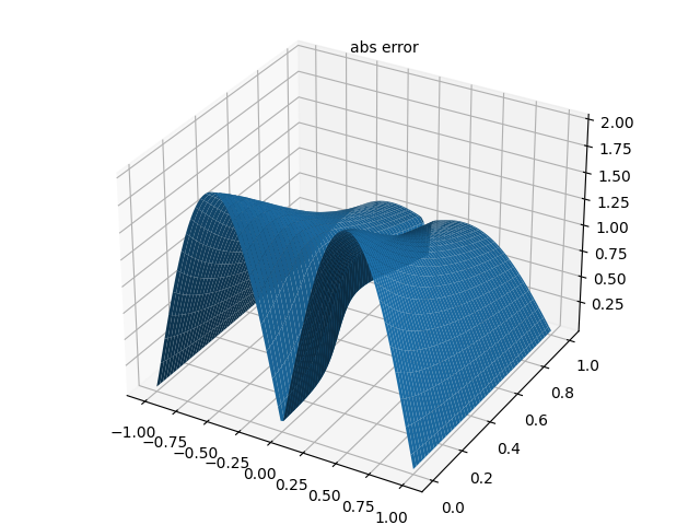
u_error = torch.abs(u_pred - u_real)
# 重塑为网格形式(可视化)
u_pred_fig = u_pred.reshape(h, h)
u_real_fig = u_real.reshape(h, h)
u_error_fig = u_error.reshape(h, h)
# 打印最大绝对误差
max_error = float(torch.max(u_error))
print(f"最大绝对误差:{max_error:.8f}")
# 创建结果保存目录
os.makedirs("result_img", exist_ok=True)
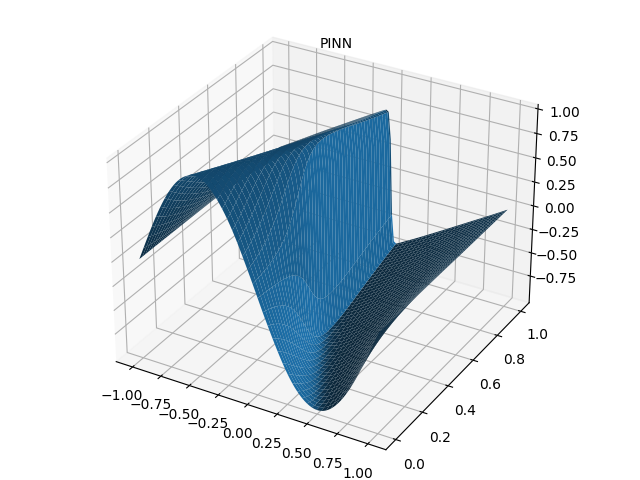
# 1. 绘制 PINN 预测结果图
fig = plt.figure(figsize=(8, 6))
ax = Axes3D(fig)
ax.plot_surface(
xm.cpu().detach().numpy(),
tm.cpu().detach().numpy(),
u_pred_fig.cpu().detach().numpy(),
cmap=cm.coolwarm
)
ax.set_xlabel('x')
ax.set_ylabel('t')
ax.set_zlabel('u')
ax.text2D(0.5, 0.9, "PINN Prediction", transform=ax.transAxes)
plt.savefig("result_img/PINN_solve.png")
plt.show()
# 2. 绘制 RK4 真实解图
fig = plt.figure(figsize=(8, 6))
ax = Axes3D(fig)
ax.plot_surface(X, T, Z, cmap=cm.coolwarm)
ax.set_xlabel('x')
ax.set_ylabel('t')
ax.set_zlabel('u')
ax.text2D(0.5, 0.9, "RK4 Numerical Solution", transform=ax.transAxes)
plt.savefig("result_img/real_solve.png")
plt.show()
# 3. 绘制绝对误差图
fig = plt.figure(figsize=(8, 6))
ax = Axes3D(fig)
ax.plot_surface(
xm.cpu().detach().numpy(),
tm.cpu().detach().numpy(),
u_error_fig.cpu().detach().numpy(),
cmap=cm.viridis
)
ax.set_xlabel('x')
ax.set_ylabel('t')
ax.set_zlabel('Absolute Error')
ax.text2D(0.5, 0.9, "Absolute Error", transform=ax.transAxes)
plt.savefig("result_img/abs_error.png")
plt.show()四、实验结果
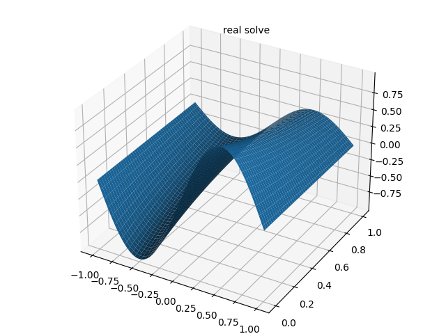
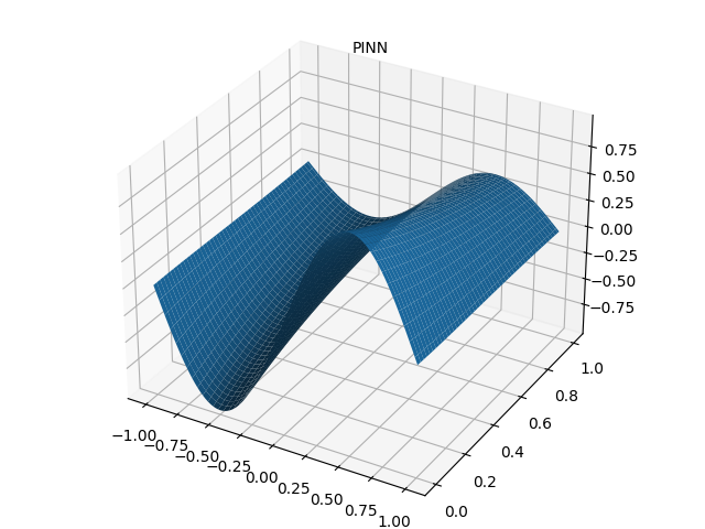
4.1 真实解(RK4 数值解)
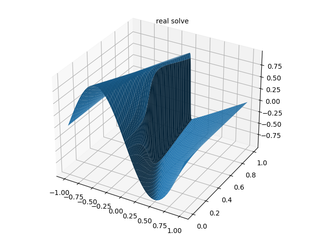
4.2 PINN 预测结果
4.3 绝对误差分布
4.4 识别的粘度系数 ν

参考文献
- PINN 解偏微分方程实例:https://blog.csdn.net/qq_49323609/article/details/139906996
- GitHub 代码仓库:https://github.com/YanxinTong/PINNs-for-PDE/tree/main/PINN_exp4_inverse_Burgers
- RK4 求解 Burgers 方程:https://blog.csdn.net/ikhui7/article/details/141927874
总结
- 偏微分方程反问题表现为方程参数/边界条件未知,需结合观测数据与物理规律反演求解,PINNs 是该类问题的有效求解方法。
- 四阶龙格-库塔法(RK4)是求解常微分方程初值问题的高精度数值方法,可用于生成 Burgers 方程的数值解以构造 PINN 训练数据。
- PINN 求解反问题通过构建包含物理损失、边界损失和数据损失的总损失函数,联合优化神经网络参数与未知物理参数,实现解函数与未知参数的同步反演。
下一合辑
- 偏微分方程 | PINN(2)-CSDN博客
https://blog.csdn.net/u013669912/article/details/159213730
reference
- 偏微分方程的正问题和逆问题 (inverse problem)_偏微分方程反问题-CSDN 博客
https://blog.csdn.net/qq_38517015/article/details/101479523 - Inverse Problems +.5ex in Partial Differential Equations - 2025NTNU.pdf
https://www.math.uni-frankfurt.de/~harrach/talks/2025NTNU.pdf - PINN for PDE(偏微分方程)1 - 正向问题_pinn 求解 pde-CSDN 博客
https://blog.csdn.net/m0_62030579/article/details/148370076 - PINN for PDE(偏微分方程)2 - 正向问题 - Diffusion_pinn 正问题求解思路-CSDN 博客
https://blog.csdn.net/m0_62030579/article/details/148370176 - PINN for PDE(偏微分方程)3 - 正向问题 - Burgers' equation_1d burgers' equation with pinn 例子-CSDN 博客
https://blog.csdn.net/m0_62030579/article/details/148370198 - PINN for PDE(偏微分方程)4 - 反向问题 - Burgers' equation_pinn 反问题-CSDN 博客
https://blog.csdn.net/m0_62030579/article/details/148370239