【多模态模型学习】从零手撕一个Vision Transformer（ViT）模型实战篇

本文主要是通过自己构建一个VIT模型完成一个简单的分类任务。

一、环境搭建

电脑配置：win10+RTX4080SX4

命令行执行以下命令，建一个虚拟环境，安装依赖库

# 创建虚拟环境
conda create -n vit python=3.10 -y
# 激活虚拟环境
conda activate vit
# 安装依赖库
pip3 install torch==2.6.0 torchvision==0.21.0 --index-url https://download.pytorch.org/whl/cu124
pip install pillow==12.1.1 matplotlib==3.10.8 einops==0.8.2 torchsummary==1.5.1

二、数据集下载

运行命令：

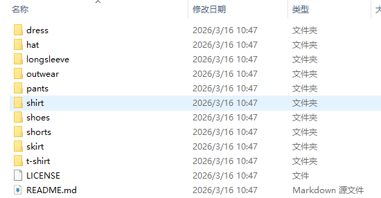
git clone https://github.com/lightly-ai/dataset_clothing_images.git my_data_dir

下载完以后删除文件夹里面的git文件，最终训练数据如图所示。

三、代码构建

（1）本地创建python文件，vit_model.py。

import torch
from torch import nn, Tensor
from torchvision.transforms import Compose, Resize, ToTensor
from einops.layers.torch import Rearrange, Reduce
from einops import repeat
from PIL import Image
from torchsummary import summary

# ===================== 1. PatchEmbedding：图像分块与嵌入 =====================
class PatchEmbedding(nn.Module):
    """
    核心作用：将224x224的RGB图像切分为16x16的Patch，映射为固定维度的向量，
    并添加CLS Token（分类专用）和位置编码（保留空间信息）
    """
    def __init__(self, 
                 in_channels: int = 3,  # 输入图像通道数（RGB=3）
                 patch_size: int = 16,  # 每个Patch的尺寸（16x16）
                 emb_size: int = 768,   # 每个Patch嵌入后的维度（ViT-Base标准）
                 img_size: int = 224):  # 输入图像尺寸
        super().__init__()
        self.patch_size = patch_size
        
        # 1. CLS Token：可学习的一维向量，拼接在所有Patch前，最终用它做分类
        # shape: [1, 1, 768]（1个token，1个batch维度，768维）
        self.cls_token = nn.Parameter(torch.randn(1, 1, emb_size))
        
        # 2. 位置编码：为每个Patch（196个）+ CLS Token（1个）分配位置向量
        # shape: [197, 768]（197个位置，每个768维），可学习
        self.positions = nn.Parameter(torch.randn((img_size // patch_size)**2 + 1, emb_size))
        
        # 3. Patch投影层：将每个16x16x3的Patch转为768维向量
        self.projection = nn.Sequential(
            # Rearrange：维度重排，把图像切分为Patch
            # 输入shape [b, 3, 224, 224] → 输出 [b, 196, 768]
            # (h s1)表示高度=h*s1，s1=patch_size，最终h=224/16=14，h*w=196个Patch
            Rearrange('b c (h s1) (w s2) -> b (h w) (s1 s2 c)', s1=patch_size, s2=patch_size),
            # Linear层：将每个Patch的像素值（16*16*3=768）映射为768维向量（维度不变，可学习）
            nn.Linear(patch_size * patch_size * in_channels, emb_size),
        )

    def forward(self, x: Tensor) -> Tensor:
        b, _, _, _ = x.shape  # 获取batch_size（b）
        x = self.projection(x)  # 第一步：图像切分+投影 → [b, 196, 768]
        
        # 复制CLS Token到整个批次：把[1,1,768] → [b,1,768]（每个样本都有CLS Token）
        cls_tokens = repeat(self.cls_token, '() n e -> b n e', b=b)
        
        # 拼接CLS Token和Patch Embedding：[b,1,768] + [b,196,768] → [b,197,768]
        x = torch.cat([cls_tokens, x], dim=1)
        
        # 添加位置编码：每个位置的向量 += 对应位置编码（保留空间信息）
        x += self.positions
        return x  # 最终输出 [b, 197, 768]

# ===================== 2. MultiHeadSelfAttention：多头自注意力 =====================
class MultiHeadSelfAttention(nn.Module):
    """
    核心作用：让每个Patch关注其他Patch的信息（包括CLS Token），捕捉全局特征
    PyTorch的MultiHeadAttention要求输入格式为 [seq_len, batch, emb_size]
    """
    def __init__(self, emb_size: int, num_heads: int = 12, dropout: float = 0.):
        super().__init__()
        # 12个头的自注意力（ViT-Base标准），每个头处理768/12=64维
        self.attention = nn.MultiheadAttention(emb_size, num_heads, dropout=dropout, batch_first=False)

    def forward(self, x: Tensor) -> Tensor:
        # 输入shape [b, 197, 768] → 转置为 [197, b, 768] 适配PyTorch接口
        x = x.transpose(0, 1)
        # 自注意力：Q=K=V=x，输出shape [197, b, 768]
        x, _ = self.attention(x, x, x)
        # 转置还原：[197, b, 768] → [b, 197, 768]
        return x.transpose(0, 1)

# ===================== 3. ResidualAdd：残差连接 =====================
class ResidualAdd(nn.Module):
    """
    核心作用：实现残差连接（Residual Connection），解决深度网络梯度消失问题
    公式：output = fn(x) + x
    """
    def __init__(self, fn):
        super().__init__()
        self.fn = fn  # 传入需要执行的子模块（如注意力/前馈网络）

    def forward(self, x: Tensor, **kwargs) -> Tensor:
        res = x  # 保存原始输入作为残差
        x = self.fn(x, **kwargs)  # 执行子模块计算
        x += res  # 残差相加
        return x

# ===================== 4. FeedForwardBlock：前馈网络 =====================
class FeedForwardBlock(nn.Sequential):
    """
    核心作用：对每个Token的特征进行非线性变换，增强模型表达能力
    结构：Linear(768→3072) → GELU → Dropout → Linear(3072→768)
    """
    def __init__(self, emb_size: int, expansion: int = 4, drop_p: float = 0.):
        super().__init__(
            # 升维：768 → 768*4=3072（扩展系数4是ViT标准）
            nn.Linear(emb_size, expansion * emb_size),
            nn.GELU(),  # 激活函数（比ReLU更平滑，ViT专用）
            nn.Dropout(drop_p),  # 防止过拟合
            # 降维：3072 → 768（还原维度，适配残差连接）
            nn.Linear(expansion * emb_size, emb_size),
        )

# ===================== 5. TransformerEncoderBlock：Transformer编码器块 =====================
class TransformerEncoderBlock(nn.Sequential):
    """
    核心作用：单个Transformer编码器块，包含「注意力+残差」和「前馈+残差」两个子模块
    结构：LayerNorm → 注意力 → Dropout → 残差 + LayerNorm → 前馈 → Dropout → 残差
    """
    def __init__(self,
                 emb_size: int = 768,
                 drop_p: float = 0.,
                 forward_expansion: int = 4,
                 forward_drop_p: float = 0.,
                 num_heads: int = 12):
        super().__init__(
            # 第一个残差块：层归一化 + 自注意力 + Dropout
            ResidualAdd(nn.Sequential(
                nn.LayerNorm(emb_size),  # 层归一化（稳定训练）
                MultiHeadSelfAttention(emb_size, num_heads=num_heads, dropout=drop_p),
                nn.Dropout(drop_p)
            )),
            # 第二个残差块：层归一化 + 前馈网络 + Dropout
            ResidualAdd(nn.Sequential(
                nn.LayerNorm(emb_size),
                FeedForwardBlock(emb_size, expansion=forward_expansion, drop_p=forward_drop_p),
                nn.Dropout(drop_p)
            ))
        )

# ===================== 6. TransformerEncoder：堆叠编码器块 =====================
class TransformerEncoder(nn.Sequential):
    """
    核心作用：堆叠多个TransformerEncoderBlock（ViT-Base堆叠12层）
    """
    def __init__(self, depth: int = 12, **kwargs):
        # 生成depth个编码器块并堆叠
        super().__init__(*[TransformerEncoderBlock(**kwargs) for _ in range(depth)])

# ===================== 7. ClassificationHead：分类头 =====================
class ClassificationHead(nn.Sequential):
    """
    核心作用：将Transformer输出的特征转为分类结果
    步骤：全局平均池化 → 层归一化 → 线性分类
    """
    def __init__(self, emb_size: int = 768, n_classes: int = 1000):
        super().__init__(
            # Reduce：对197个Token做平均池化，[b,197,768] → [b,768]
            Reduce('b n e -> b e', reduction='mean'),
            nn.LayerNorm(emb_size),  # 归一化
            nn.Linear(emb_size, n_classes)  # 768维 → 分类类别数（如10类）
        )

# ===================== 8. ViT：完整模型 =====================
class ViT(nn.Sequential):
    """
    核心作用：整合所有模块，形成完整的Vision Transformer
    流程：PatchEmbedding → TransformerEncoder → ClassificationHead
    """
    def __init__(self,
                 in_channels: int = 3,
                 patch_size: int = 16,
                 emb_size: int = 768,
                 img_size: int = 224,
                 depth: int = 12,  # 编码器块数量（ViT-Base=12）
                 n_classes: int = 1000,
                 **kwargs):
        super().__init__(
            PatchEmbedding(in_channels, patch_size, emb_size, img_size),  # 分块+嵌入
            TransformerEncoder(depth, emb_size=emb_size, **kwargs),      # 特征提取
            ClassificationHead(emb_size, n_classes)                      # 分类
        )

# ===================== 9. 运行测试 =====================
if __name__ == "__main__":
    # 1. 图像预处理：读取→Resize→转Tensor（适配ViT输入）
    img_path = "01.jpg"  # 替换为你的图像路径
    img = Image.open(img_path).convert("RGB")  # 确保RGB格式（避免灰度图报错）
    transform = Compose([Resize((224, 224)), ToTensor()])  # 转为224x224的张量
    x = transform(img)  # 输出shape [3, 224, 224]
    x = x.unsqueeze(0)  # 添加batch维度 → [1, 3, 224, 224]
    print(f"输入图像张量形状: {x.shape}")

    # 2. 初始化模型：分类类别数设为10（可根据需求修改）
    vit_model = ViT(n_classes=10)
    print("\n=== ViT模型结构 ===")
    # 打印模型结构和参数：输入尺寸(3,224,224)，batch_size=1
    summary(vit_model, input_size=(3, 224, 224), batch_size=1, device="cpu")

    # 3. 模型推理（评估模式，禁用梯度计算提升速度）
    vit_model.eval()  # 切换到评估模式（Dropout等层失效）
    with torch.no_grad():
        output = vit_model(x)  # 前向传播 → [1, 10]（1个样本，10类概率）
        probabilities = torch.softmax(output, dim=1)  # 转为概率（总和=1）
        predicted_class = torch.argmax(probabilities, dim=1).item()  # 取概率最大的类别

    # 4. 输出结果
    print(f"\n模型输出形状: {output.shape}")
    print(f"预测类别索引: {predicted_class}")
    print(f"预测类别概率: {probabilities[0][predicted_class]:.4f}")

（2）本地创建python文件，vit_train.py。

import torch
import torch.nn as nn
import torch.optim as optim
from torch.utils.data import DataLoader, random_split
from torchvision.datasets import ImageFolder
from torchvision.transforms import Compose, Resize, ToTensor, Normalize
from vit_model import ViT  # 

# ===================== 1. 基础配置 =====================
# 设置设备
device = torch.device('cuda' if torch.cuda.is_available() else 'cpu')
print(f'使用设备: {device}')

# 训练超参数（集中管理，方便修改）
CONFIG = {
    "BATCH_SIZE": 16,
    "EPOCHS": 50,
    "IMG_SIZE": 224,
    "LEARNING_RATE": 3e-4,
    "DATA_PATH": "my_data_dir",  # 你的数据集根目录
    "VAL_SPLIT_RATIO": 0.1,      # 验证集比例（10%）
    "SAVE_MODEL_PATH": "vit_classifier.pth",
    "CLASSES_PATH": "classes.txt"  # 保存类别列表的文件
}

# ===================== 2. 数据加载与划分 =====================
def load_and_split_data(data_path, img_size=224, batch_size=32, val_ratio=0.1):
    """
    加载数据集并按9:1划分训练集/验证集
    :param data_path: 数据集根目录（按类别分文件夹）
    :param img_size: 图像尺寸
    :param batch_size: 批次大小
    :param val_ratio: 验证集比例
    :return: 训练加载器、验证加载器、类别列表
    """
    # 数据预处理
    transform = Compose([
        Resize((img_size, img_size)),
        ToTensor(),
        Normalize(mean=[0.485, 0.456, 0.406],
                  std=[0.229, 0.224, 0.225])
    ])
    
    # 加载完整数据集
    full_dataset = ImageFolder(root=data_path, transform=transform)
    classes = full_dataset.classes  # 获取类别列表
    
    # 保存类别列表（供测试代码使用）
    with open(CONFIG["CLASSES_PATH"], 'w', encoding='utf-8') as f:
        f.write('\n'.join(classes))
    print(f"类别列表已保存到: {CONFIG['CLASSES_PATH']}")
    
    # 打印数据集信息
    print(f"数据集总样本数: {len(full_dataset)}")
    print(f"类别数: {len(classes)}, 类别: {classes}")
    
    # 划分训练集和验证集
    val_size = int(len(full_dataset) * val_ratio)
    train_size = len(full_dataset) - val_size
    train_dataset, val_dataset = random_split(full_dataset, [train_size, val_size])
    print(f"训练集样本数: {len(train_dataset)}, 验证集样本数: {len(val_dataset)}")
    
    # 创建数据加载器
    train_loader = DataLoader(
        train_dataset, 
        batch_size=batch_size, 
        shuffle=True,
        num_workers=0,
        #pin_memory=True if device.type == 'cuda' else False
        pin_memory=False
    )
    val_loader = DataLoader(
        val_dataset, 
        batch_size=batch_size, 
        shuffle=False,
        num_workers=0,
        #pin_memory=True if device.type == 'cuda' else False
        pin_memory=False
    )
    
    return train_loader, val_loader, classes

# ===================== 3. 训练与验证函数 =====================
def train_one_epoch(model, train_loader, criterion, optimizer, device):
    """训练一个epoch，返回训练损失和准确率"""
    model.train()
    total_loss = 0.0
    correct = 0
    total = 0
    
    for batch_idx, (images, labels) in enumerate(train_loader):
        images, labels = images.to(device), labels.to(device)
        
        # 前向传播
        outputs = model(images)
        loss = criterion(outputs, labels)
        
        # 反向传播
        optimizer.zero_grad()
        loss.backward()
        torch.nn.utils.clip_grad_norm_(model.parameters(), max_norm=1.0)
        optimizer.step()
        
        # 统计指标
        total_loss += loss.item()
        _, predicted = outputs.max(1)
        total += labels.size(0)
        correct += predicted.eq(labels).sum().item()
        
        # 每10个批次打印一次进度
        if (batch_idx + 1) % 10 == 0:
            batch_acc = 100. * correct / total
            print(f"  批次 {batch_idx+1}/{len(train_loader)} | 批次损失: {loss.item():.4f} | 批次准确率: {batch_acc:.2f}%")
    
    epoch_loss = total_loss / len(train_loader)
    epoch_acc = 100. * correct / total
    return epoch_loss, epoch_acc

def validate(model, val_loader, criterion, device):
    """验证一个epoch，返回验证损失和准确率"""
    model.eval()
    total_loss = 0.0
    correct = 0
    total = 0
    
    with torch.no_grad():
        for images, labels in val_loader:
            images, labels = images.to(device), labels.to(device)
            
            outputs = model(images)
            loss = criterion(outputs, labels)
            
            total_loss += loss.item()
            _, predicted = outputs.max(1)
            total += labels.size(0)
            correct += predicted.eq(labels).sum().item()
    
    val_loss = total_loss / len(val_loader)
    val_acc = 100. * correct / total
    return val_loss, val_acc

# ===================== 4. 主训练流程 =====================
def main():
    # 1. 加载数据
    train_loader, val_loader, classes = load_and_split_data(
        data_path=CONFIG["DATA_PATH"],
        img_size=CONFIG["IMG_SIZE"],
        batch_size=CONFIG["BATCH_SIZE"],
        val_ratio=CONFIG["VAL_SPLIT_RATIO"]
    )
    
    # 2. 创建模型
    model = ViT(
        in_channels=3,
        patch_size=16,
        emb_size=768,
        img_size=CONFIG["IMG_SIZE"],
        depth=12,
        n_classes=len(classes),
        num_heads=12,
        drop_p=0.1,
        forward_drop_p=0.1
    ).to(device)
    print("\n==================== 模型信息 ====================")
    print(f"模型总参数量: {sum(p.numel() for p in model.parameters()):,}")
    
    # 3. 定义损失函数和优化器
    criterion = nn.CrossEntropyLoss()
    optimizer = optim.AdamW(
        model.parameters(),
        lr=CONFIG["LEARNING_RATE"],
        weight_decay=0.01
    )
    
    # 4. 开始训练
    print("\n==================== 开始训练 ====================")
    best_val_acc = 0.0
    for epoch in range(CONFIG["EPOCHS"]):
        # 训练
        train_loss, train_acc = train_one_epoch(model, train_loader, criterion, optimizer, device)
        
        # 验证
        val_loss, val_acc = validate(model, val_loader, criterion, device)
        
        # 打印epoch结果
        print(f"\nEpoch {epoch+1}/{CONFIG['EPOCHS']}")
        print(f"训练损失: {train_loss:.4f} | 训练准确率: {train_acc:.2f}%")
        print(f"验证损失: {val_loss:.4f} | 验证准确率: {val_acc:.2f}%")
        
        # 保存最佳模型
        if val_acc > best_val_acc:
            best_val_acc = val_acc
            torch.save(model.state_dict(), CONFIG["SAVE_MODEL_PATH"])
            print(f"保存最佳模型（验证准确率: {best_val_acc:.2f}%）到 {CONFIG['SAVE_MODEL_PATH']}")
    
    print("\n==================== 训练完成 ====================")
    print(f"最佳验证准确率: {best_val_acc:.2f}%")
    print(f"模型保存路径: {CONFIG['SAVE_MODEL_PATH']}")
    print(f"类别列表保存路径: {CONFIG['CLASSES_PATH']}")

if __name__ == '__main__':
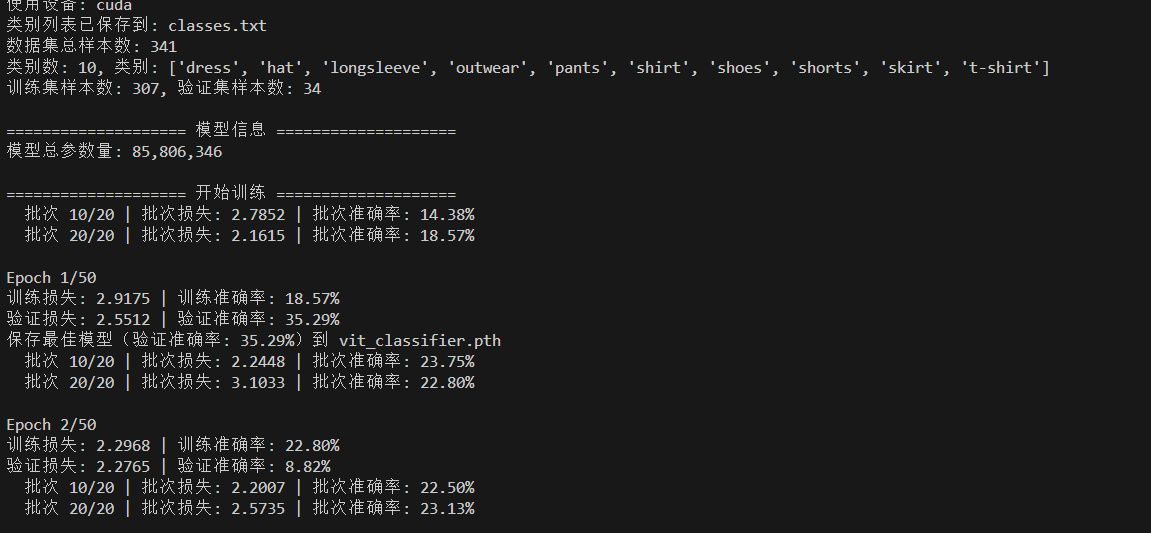
    main()

训练过程如下：

（2）本地创建python文件，vit_test.py。

import torch
import torch.nn as nn
from torchvision.transforms import Compose, Resize, ToTensor, Normalize
from PIL import Image
# 导入ViT模型（和训练代码保持一致）
from vit_model import ViT  # 若之前的类名是ViT_model，这里改为ViT_model

# ===================== 1. 配置参数 =====================
# 设置设备
device = torch.device('cuda' if torch.cuda.is_available() else 'cpu')
print(f'使用设备: {device}')

# 测试配置（需和训练时保持一致）
TEST_CONFIG = {
    "IMG_SIZE": 224,
    "MODEL_PATH": "vit_classifier.pth",  # 训练好的模型路径
    "CLASSES_PATH": "classes.txt",       # 保存类别列表的文件
    "TEST_IMAGES": ["01.jpg", "02.jpg"]  # 需要预测的图片路径
}

# ===================== 2. 加载类别列表 =====================
def load_classes(classes_path):
    """加载训练时保存的类别列表"""
    with open(classes_path, 'r', encoding='utf-8') as f:
        classes = [line.strip() for line in f if line.strip()]
    print(f"加载类别列表: {classes}")
    return classes

# ===================== 3. 加载模型 =====================
def load_model(model_path, classes, img_size=224, device=device):
    """加载训练好的ViT模型"""
    # 创建模型结构（参数需和训练时完全一致）
    model = ViT(
        in_channels=3,
        patch_size=16,
        emb_size=768,
        img_size=img_size,
        depth=12,
        n_classes=len(classes),
        num_heads=12,
        drop_p=0.1,
        forward_drop_p=0.1
    ).to(device)
    
    # 加载模型权重
    model.load_state_dict(torch.load(model_path, map_location=device))
    model.eval()  # 切换到评估模式
    print(f"模型加载完成: {model_path}")
    return model

# ===================== 4. 单张图片预测 =====================
def predict_single_image(model, image_path, classes, img_size=224, device=device):
    """
    单张图片预测
    :param model: 训练好的模型
    :param image_path: 图片路径
    :param classes: 类别列表
    :param img_size: 图像尺寸
    :param device: 设备
    """
    # 数据预处理（必须和训练时完全一致）
    transform = Compose([
        Resize((img_size, img_size)),
        ToTensor(),
        Normalize(mean=[0.485, 0.456, 0.406],
                  std=[0.229, 0.224, 0.225])
    ])
    
    try:
        # 加载并处理图片
        image = Image.open(image_path).convert('RGB')
        image_tensor = transform(image).unsqueeze(0).to(device)  # 添加batch维度
        
        # 预测
        with torch.no_grad():
            outputs = model(image_tensor)
            probabilities = torch.softmax(outputs, dim=1)  # 转为概率
            predicted_idx = torch.argmax(probabilities, dim=1).item()  # 预测类别索引
            confidence = probabilities[0][predicted_idx].item()  # 置信度
        
        # 打印结果
        print("\n==================== 预测结果 ====================")
        print(f"图片路径: {image_path}")
        print(f"预测类别: {classes[predicted_idx]}")
        print(f"置信度: {confidence:.2%}")
        
        # 可选：打印前3个高置信度的类别
        top3_probs, top3_idxs = torch.topk(probabilities, 3, dim=1)
        print("前3个高置信度类别:")
        for i in range(3):
            print(f"  {classes[top3_idxs[0][i].item()]}: {top3_probs[0][i].item():.2%}")
            
    except Exception as e:
        print(f"预测图片 {image_path} 失败: {str(e)}")

# ===================== 5. 批量预测 =====================
def batch_predict(model, image_paths, classes, img_size=224, device=device):
    """批量预测多张图片"""
    print("\n==================== 开始批量预测 ====================")
    for img_path in image_paths:
        predict_single_image(model, img_path, classes, img_size, device)

# ===================== 主测试流程 =====================
def main():
    # 1. 加载类别列表
    classes = load_classes(TEST_CONFIG["CLASSES_PATH"])
    
    # 2. 加载模型
    model = load_model(TEST_CONFIG["MODEL_PATH"], classes, TEST_CONFIG["IMG_SIZE"], device)
    
    # 3. 批量预测
    batch_predict(model, TEST_CONFIG["TEST_IMAGES"], classes, TEST_CONFIG["IMG_SIZE"], device)

if __name__ == '__main__':
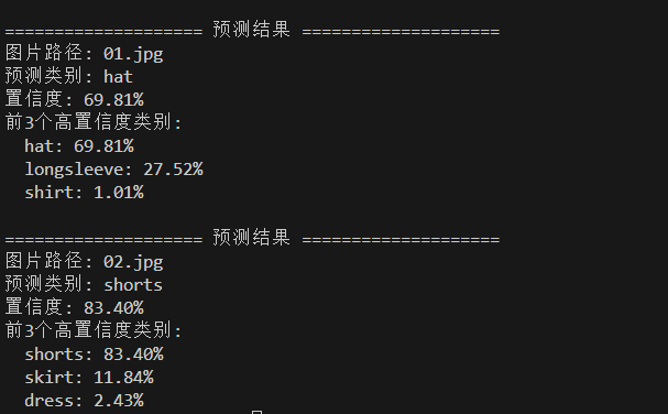
    main()

测试图像01.jpg：

测试图像02.jpg：

测试结果：