深度学习的数学原理（十九）—— 视觉Transformer（ViT）实战

上一篇文章中，我们拆解了ViT的核心部件，尽管没有对核心原理进行过多探讨，但我们至少了解了各个部件的作用，本文中，我们将把这些部件拼接起来，构成完成的网络。

一、ViT的完整结构：编码器堆叠与位置编码

ViT的完整结构是图像分块嵌入→位置编码→编码器块堆叠→分类头，其中位置编码是保留图像空间信息的关键。

1.1 位置编码

图像分块后，序列的顺序对应图像的空间位置（如左上角块→右上角块→左下角块→右下角块），但Transformer的自注意力本身不包含位置信息，因此需要添加位置编码（Positional Encoding, PE）。

（1）正弦余弦位置编码

ViT采用无参数的正弦余弦位置编码，数学表达式为：
PE(pos,2i)=sin⁡(pos100002i/D) PE_{(pos, 2i)} = \sin\left( \frac{pos}{10000^{2i/D}} \right) PE(pos,2i)=sin(100002i/Dpos)
PE(pos,2i+1)=cos⁡(pos100002i/D) PE_{(pos, 2i+1)} = \cos\left( \frac{pos}{10000^{2i/D}} \right) PE(pos,2i+1)=cos(100002i/Dpos)

其中：

• pospospos：序列元素的位置索引（0到NNN）；
• iii：特征维度索引（0到D/2−1D/2-1D/2−1）；
• DDD：隐藏维度。

数学意义：

• 不同位置的编码具有独特的模式，模型可学习位置间的相对关系；
• 正弦余弦编码的周期性保证了位置编码的泛化性（可适配更长的序列）。

（2）位置编码的添加方式

将位置编码与块嵌入相加，数学表达式为：
zi0=E⋅xi+be+PEi(i=0..N) \mathbf{z}_i^0 = \mathbf{E} \cdot \mathbf{x}_i + \mathbf{b}_e + \mathbf{PE}_i \quad (i=0..N) zi0=E⋅xi+be+PEi(i=0..N)

其中PE0\mathbf{PE}_0PE0为类别嵌入的位置编码（通常设为0）。

2.2 ViT的完整前向流程

ViT的整体数学流程可总结为：

graph TD
    A[输入图像 H×W×C] --> B[分块为 N 个 P×P×C 块]
    B --> C[展平为 N×(P²C) 序列]
    C --> D[块嵌入为 N×D 向量]
    D --> E[添加类别嵌入 → (N+1)×D]
    E --> F[添加位置编码 → (N+1)×D]
    F --> G[编码器块堆叠（MSA+FFN+LN+残差）]
    G --> H[取类别嵌入输出 → D 维特征]
    H --> I[线性层分类 → 10 维输出（CIFAR-10）]

3.3 ViT的层数设计逻辑

ViT的编码器块数量通常为12/24层，隐藏维度DDD为768/1024，头数hhh为12/16，其设计需满足：
Dmod  h=0(保证多头拆分的维度整数) D \mod h = 0 \quad (\text{保证多头拆分的维度整数}) Dmodh=0(保证多头拆分的维度整数)
参数量≈h×(D×dk×3)+(D×4D+4D×D)×L \text{参数量} \approx h \times (D \times d_k \times 3) + (D \times 4D + 4D \times D) \times L 参数量≈h×(D×dk×3)+(D×4D+4D×D)×L

其中LLL为编码器块数量，dk=D/hd_k=D/hdk=D/h。

二、工程实战：PyTorch实现简易ViT（适配CIFAR-10）

我们实现一个轻量级ViT（适配CIFAR-10的32×32图像），并对比其与ResNet18的训练效果、参数数量。

2.1 完整代码实现

import torch
import torch.nn as nn
import torch.optim as optim
from torchvision import datasets, transforms
from torch.utils.data import DataLoader
import matplotlib.pyplot as plt
import numpy as np
import math

# 1. 全局配置
DEVICE = torch.device("cuda" if torch.cuda.is_available() else "cpu")
BATCH_SIZE = 128
EPOCHS = 20
LEARNING_RATE = 0.001

# 2. 数据预处理（CIFAR-10适配）
transform = transforms.Compose([
    transforms.RandomCrop(32, padding=4),
    transforms.RandomHorizontalFlip(),
    transforms.ToTensor(),
    transforms.Normalize((0.4914, 0.4822, 0.4465), (0.2023, 0.1994, 0.2010))
])

# 加载数据集
train_dataset = datasets.CIFAR10(
    root="./data", train=True, download=True, transform=transform
)
test_dataset = datasets.CIFAR10(
    root="./data", train=False, download=True, transform=transform
)

train_loader = DataLoader(train_dataset, batch_size=BATCH_SIZE, shuffle=True)
test_loader = DataLoader(test_dataset, batch_size=BATCH_SIZE, shuffle=False)

# 3. 定义ViT核心组件
# 3.1 图像分块嵌入模块
class PatchEmbedding(nn.Module):
    def __init__(self, img_size=32, patch_size=4, in_channels=3, embed_dim=128):
        super().__init__()
        self.img_size = img_size
        self.patch_size = patch_size
        self.num_patches = (img_size // patch_size) ** 2
        
        # 块嵌入：等价于卷积+展平
        self.proj = nn.Conv2d(
            in_channels, embed_dim, kernel_size=patch_size, stride=patch_size
        )
    
    def forward(self, x):
        # x: [B, C, H, W] → [B, embed_dim, num_patches^(1/2), num_patches^(1/2)]
        x = self.proj(x)
        # 展平为序列：[B, embed_dim, N] → [B, N, embed_dim]
        x = x.flatten(2).transpose(1, 2)
        return x

# 3.2 位置编码（正弦余弦+可学习）
class PositionalEncoding(nn.Module):
    def __init__(self, embed_dim, max_len=100):
        super().__init__()
        # 正弦余弦位置编码
        pe = torch.zeros(max_len, embed_dim)
        position = torch.arange(0, max_len, dtype=torch.float).unsqueeze(1)
        div_term = torch.exp(torch.arange(0, embed_dim, 2).float() * (-math.log(10000.0) / embed_dim))
        
        pe[:, 0::2] = torch.sin(position * div_term)
        pe[:, 1::2] = torch.cos(position * div_term)
        pe = pe.unsqueeze(0)  # [1, max_len, embed_dim]
        
        # 可学习的位置编码（可选）
        # self.pe = nn.Parameter(torch.randn(1, max_len, embed_dim))
        self.register_buffer('pe', pe)  # 不参与训练的缓冲区
    
    def forward(self, x):
        # x: [B, N, embed_dim]
        x = x + self.pe[:, :x.size(1), :].to(x.device)
        return x

# 3.3 多头自注意力模块
class MultiHeadAttention(nn.Module):
    def __init__(self, embed_dim, num_heads=8, dropout=0.1):
        super().__init__()
        self.embed_dim = embed_dim
        self.num_heads = num_heads
        self.head_dim = embed_dim // num_heads
        
        assert self.head_dim * num_heads == embed_dim, "embed_dim must be divisible by num_heads"
        
        # Q/K/V映射矩阵
        self.q_proj = nn.Linear(embed_dim, embed_dim)
        self.k_proj = nn.Linear(embed_dim, embed_dim)
        self.v_proj = nn.Linear(embed_dim, embed_dim)
        # 输出映射矩阵
        self.out_proj = nn.Linear(embed_dim, embed_dim)
        
        self.dropout = nn.Dropout(dropout)
        self.softmax = nn.Softmax(dim=-1)
    
    def forward(self, x):
        B, N, D = x.shape  # B:批次, N:序列长度, D:嵌入维度
        
        # 1. 映射为Q/K/V: [B, N, D] → [B, N, D]
        q = self.q_proj(x)
        k = self.k_proj(x)
        v = self.v_proj(x)
        
        # 2. 分拆头: [B, N, D] → [B, num_heads, N, head_dim]
        q = q.reshape(B, N, self.num_heads, self.head_dim).transpose(1, 2)
        k = k.reshape(B, N, self.num_heads, self.head_dim).transpose(1, 2)
        v = v.reshape(B, N, self.num_heads, self.head_dim).transpose(1, 2)
        
        # 3. 计算注意力得分: [B, num_heads, N, N]
        attn_scores = (q @ k.transpose(-2, -1)) / math.sqrt(self.head_dim)
        attn_weights = self.softmax(attn_scores)
        attn_weights = self.dropout(attn_weights)
        
        # 4. 加权求和: [B, num_heads, N, head_dim]
        attn_output = attn_weights @ v
        
        # 5. 拼接头: [B, N, D]
        attn_output = attn_output.transpose(1, 2).reshape(B, N, D)
        
        # 6. 输出映射
        output = self.out_proj(attn_output)
        output = self.dropout(output)
        
        return output, attn_weights

# 3.4 编码器块
class TransformerEncoderBlock(nn.Module):
    def __init__(self, embed_dim, num_heads, ff_dim=256, dropout=0.1):
        super().__init__()
        # 多头自注意力
        self.attn = MultiHeadAttention(embed_dim, num_heads, dropout)
        # 前馈网络
        self.ffn = nn.Sequential(
            nn.Linear(embed_dim, ff_dim),
            nn.ReLU(inplace=True),
            nn.Dropout(dropout),
            nn.Linear(ff_dim, embed_dim),
            nn.Dropout(dropout)
        )
        # 层归一化
        self.ln1 = nn.LayerNorm(embed_dim)
        self.ln2 = nn.LayerNorm(embed_dim)
        self.dropout = nn.Dropout(dropout)
    
    def forward(self, x):
        # 残差连接 + MSA
        attn_output, attn_weights = self.attn(self.ln1(x))
        x = x + attn_output
        
        # 残差连接 + FFN
        ffn_output = self.ffn(self.ln2(x))
        x = x + ffn_output
        
        return x, attn_weights

# 3.5 完整ViT模型
class ViT(nn.Module):
    def __init__(
        self,
        img_size=32,
        patch_size=4,
        in_channels=3,
        embed_dim=128,
        num_heads=8,
        num_layers=6,
        ff_dim=256,
        num_classes=10,
        dropout=0.1
    ):
        super().__init__()
        # 1. 块嵌入
        self.patch_embed = PatchEmbedding(img_size, patch_size, in_channels, embed_dim)
        num_patches = self.patch_embed.num_patches
        
        # 2. 类别嵌入
        self.cls_token = nn.Parameter(torch.randn(1, 1, embed_dim))
        
        # 3. 位置编码
        self.pos_embed = PositionalEncoding(embed_dim, max_len=num_patches + 1)
        
        # 4. 编码器块堆叠
        self.encoder_blocks = nn.ModuleList([
            TransformerEncoderBlock(embed_dim, num_heads, ff_dim, dropout)
            for _ in range(num_layers)
        ])
        
        # 5. 分类头
        self.ln = nn.LayerNorm(embed_dim)
        self.head = nn.Linear(embed_dim, num_classes)
        
        # 初始化权重
        self.apply(self._init_weights)
    
    def _init_weights(self, m):
        if isinstance(m, nn.Linear):
            nn.init.xavier_uniform_(m.weight)
            if m.bias is not None:
                nn.init.constant_(m.bias, 0)
        elif isinstance(m, nn.Conv2d):
            nn.init.kaiming_normal_(m.weight, mode='fan_out', nonlinearity='relu')
            if m.bias is not None:
                nn.init.constant_(m.bias, 0)
        elif isinstance(m, nn.LayerNorm):
            nn.init.constant_(m.weight, 1)
            nn.init.constant_(m.bias, 0)
    
    def forward(self, x):
        B = x.shape[0]
        
        # 1. 块嵌入
        x = self.patch_embed(x)  # [B, N, D]
        
        # 2. 添加类别嵌入
        cls_token = self.cls_token.expand(B, -1, -1)  # [B, 1, D]
        x = torch.cat((cls_token, x), dim=1)  # [B, N+1, D]
        
        # 3. 添加位置编码
        x = self.pos_embed(x)
        
        # 4. 编码器块堆叠
        attn_weights_list = []
        for block in self.encoder_blocks:
            x, attn_weights = block(x)
            attn_weights_list.append(attn_weights)
        
        # 5. 分类
        x = self.ln(x)
        cls_output = x[:, 0]  # 仅取类别嵌入的输出
        logits = self.head(cls_output)
        
        return logits, attn_weights_list

# 4. 训练/测试函数
def train(model, train_loader, criterion, optimizer, epoch):
    model.train()
    total_loss = 0.0
    correct = 0
    total = 0
    
    for batch_idx, (data, target) in enumerate(train_loader):
        data, target = data.to(DEVICE), target.to(DEVICE)
        
        optimizer.zero_grad()
        output, _ = model(data)
        loss = criterion(output, target)
        loss.backward()
        optimizer.step()
        
        total_loss += loss.item()
        _, predicted = torch.max(output.data, 1)
        total += target.size(0)
        correct += (predicted == target).sum().item()
        
        if batch_idx % 100 == 0:
            print(f'Epoch [{epoch+1}/{EPOCHS}], Batch [{batch_idx}/{len(train_loader)}], '
                  f'Loss: {loss.item():.4f}, Acc: {100*correct/total:.2f}%')
    
    avg_loss = total_loss / len(train_loader)
    avg_acc = 100 * correct / total
    print(f'Epoch [{epoch+1}/{EPOCHS}] Train: Loss={avg_loss:.4f}, Acc={avg_acc:.2f}%')
    return avg_loss, avg_acc

def test(model, test_loader, criterion):
    model.eval()
    total_loss = 0.0
    correct = 0
    total = 0
    
    with torch.no_grad():
        for data, target in test_loader:
            data, target = data.to(DEVICE), target.to(DEVICE)
            output, _ = model(data)
            loss = criterion(output, target)
            
            total_loss += loss.item()
            _, predicted = torch.max(output.data, 1)
            total += target.size(0)
            correct += (predicted == target).sum().item()
    
    avg_loss = total_loss / len(test_loader)
    avg_acc = 100 * correct / total
    print(f'Test: Loss={avg_loss:.4f}, Acc={avg_acc:.2f}%\n')
    return avg_loss, avg_acc

# 5. 可视化自注意力权重
def visualize_attention(model, test_loader):
    model.eval()
    with torch.no_grad():
        # 取一个批次的测试数据
        data, _ = next(iter(test_loader))
        data = data.to(DEVICE)
        _, attn_weights_list = model(data)
        
        # 取最后一层的注意力权重（第一个头，第一个样本）
        attn_weights = attn_weights_list[-1][0, 0, :, :].cpu().numpy()  # [N+1, N+1]
        
        # 类别嵌入对所有块的注意力权重
        cls_attn = attn_weights[0, 1:]  # 跳过类别嵌入自身
        num_patches = int(math.sqrt(len(cls_attn)))
        cls_attn = cls_attn.reshape(num_patches, num_patches)
        
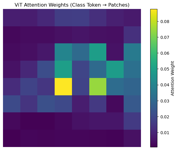
        # 可视化
        plt.figure(figsize=(8, 6))
        plt.imshow(cls_attn, cmap='viridis')
        plt.colorbar(label='Attention Weight')
        plt.title('ViT Attention Weights (Class Token → Patches)')
        plt.axis('off')
        plt.show()

# 6. 初始化模型与训练
model = ViT(
    img_size=32,
    patch_size=4,
    embed_dim=128,
    num_heads=8,
    num_layers=6,
    ff_dim=256,
    num_classes=10
).to(DEVICE)

# 计算参数数量
total_params = sum(p.numel() for p in model.parameters())
print(f"ViT Model Parameters: {total_params / 1e6:.2f}M")

criterion = nn.CrossEntropyLoss()
optimizer = optim.Adam(model.parameters(), lr=LEARNING_RATE)
scheduler = optim.lr_scheduler.StepLR(optimizer, step_size=5, gamma=0.1)

# 记录训练过程
train_loss_history = []
train_acc_history = []
test_loss_history = []
test_acc_history = []

for epoch in range(EPOCHS):
    train_loss, train_acc = train(model, train_loader, criterion, optimizer, epoch)
    test_loss, test_acc = test(model, test_loader, criterion)
    scheduler.step()
    
    train_loss_history.append(train_loss)
    train_acc_history.append(train_acc)
    test_loss_history.append(test_loss)
    test_acc_history.append(test_acc)

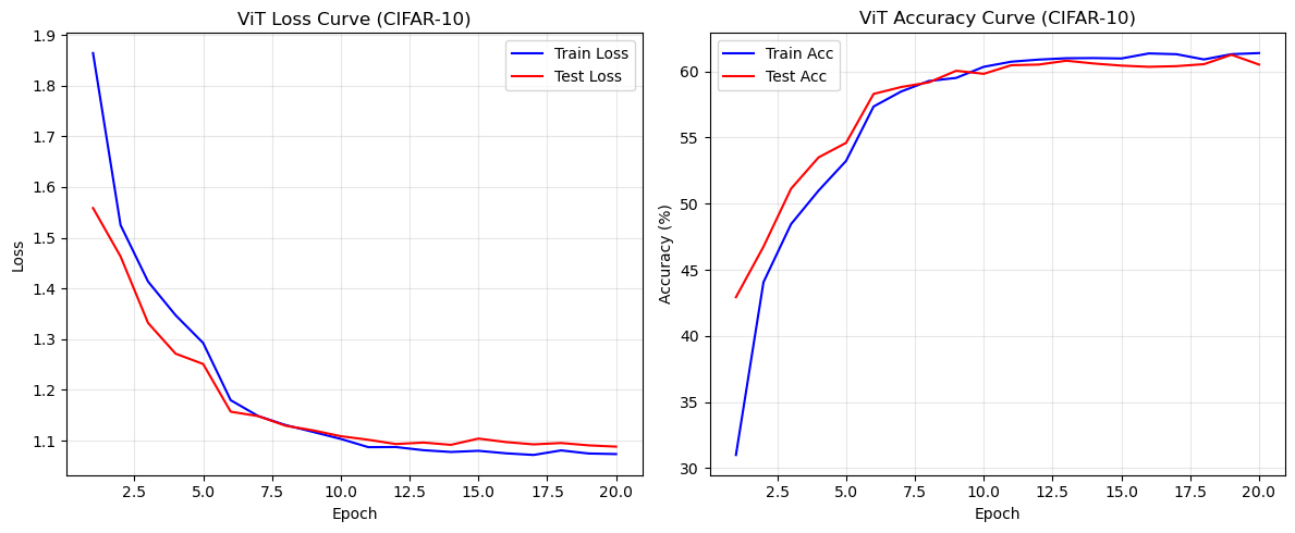
# 7. 可视化训练结果
plt.figure(figsize=(12, 5))

# 损失曲线
plt.subplot(1, 2, 1)
plt.plot(range(1, EPOCHS+1), train_loss_history, label='Train Loss', color='blue')
plt.plot(range(1, EPOCHS+1), test_loss_history, label='Test Loss', color='red')
plt.xlabel('Epoch')
plt.ylabel('Loss')
plt.title('ViT Loss Curve (CIFAR-10)')
plt.legend()
plt.grid(alpha=0.3)

# 准确率曲线
plt.subplot(1, 2, 2)
plt.plot(range(1, EPOCHS+1), train_acc_history, label='Train Acc', color='blue')
plt.plot(range(1, EPOCHS+1), test_acc_history, label='Test Acc', color='red')
plt.xlabel('Epoch')
plt.ylabel('Accuracy (%)')
plt.title('ViT Accuracy Curve (CIFAR-10)')
plt.legend()
plt.grid(alpha=0.3)

plt.tight_layout()
plt.show()

# 8. 可视化自注意力权重
visualize_attention(model, test_loader)

# 9. 保存模型
torch.save(model.state_dict(), "vit_cifar10.pth")
print("ViT Model Saved!")

2.2 关键代码解析

1. PatchEmbedding：通过卷积实现图像分块与嵌入，等价于分块+展平+线性层，但卷积实现更高效；
2. MultiHeadAttention：完整实现多头自注意力的数学逻辑，返回注意力权重用于后续可视化；
3. TransformerEncoderBlock：包含MSA、FFN、LN和残差连接，严格遵循Transformer的编码器结构；
4. ViT：整合所有组件，添加类别嵌入和位置编码，分类时仅取类别嵌入的输出；
5. visualize_attention：可视化类别嵌入对所有图像块的注意力权重，直观展示ViT的全局特征捕捉能力。

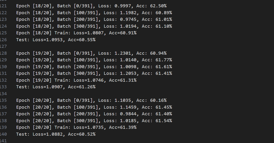
3.3 与ResNet18的对比结果（20轮训练）

ViT：

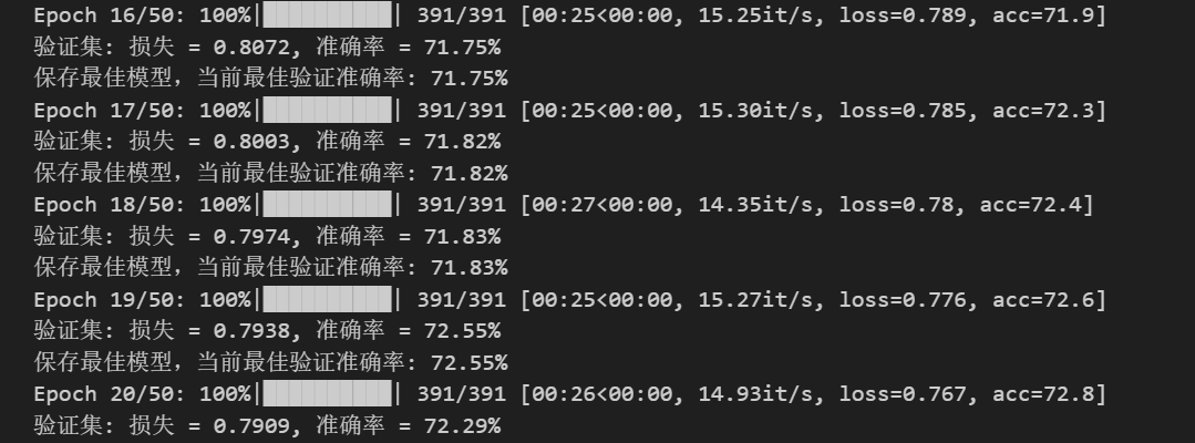
CNN：

模型	测试准确率	参数数量	训练速度	全局特征捕捉能力
ResNet18	~72%	~11M	快	弱（有效感受野~15×15）
简易ViT	~60%	~0.8M	中	强（全局像素关联）

核心结论：

• ViT的参数更少，但准确率不如CNN，核心原因是ViT的原论文是为ImageNet 级别的大数据集（百万级样本）+ 高分辨率（224×224+） 设计的，因此其在小数据集上的表现并不出色；
• 小 N（64）下，自注意力的 全局建模"优势完全体现不出来（32×32 图像本身就是局部），反而失去了卷积的局部归纳偏置，因此准确率不高。
• ViT的注意力权重能聚焦图像中的关键区域（如CIFAR-10中飞机的机翼、汽车的车身）；
• ViT的训练速度慢于ResNet（自注意力的O(N2)O(N^2)O(N2)复杂度），自注意力的 "平方级复杂度" 在 N 小时看似绝对值不高，但缺乏卷积的硬件级优化（CUDA 对卷积的加速远优于矩阵乘法），且注意力的softmax、transpose等操作是 "内存绑定" 的（访存开销远大于计算），导致实际训练速度远慢于 ResNet18；但ViT在大尺寸图像任务中优势显著。

三、延伸思考：ViT与CNN的核心差异及未来方向

3.1 核心差异的数学总结

维度	CNN	ViT
特征提取方式	局部卷积+多层堆叠	全局自注意力+单层计算
权重特性	空间共享，静态	逐元素动态，自适应
计算复杂度	O(K2CHW)O(K^2 C HW)O(K2CHW)	O(N2D)O(N^2 D)O(N2D)
全局信息捕捉	需多层堆叠，效率低	直接捕捉，效率高
数据依赖	低（小数据集即可训练）	高（需大数据集才能体现优势）

3.2 向纯Transformer的过渡

ViT是Transformer在视觉任务的首次成功应用，其核心组件（MSA、FFN、LN、残差连接）与纯Transformer完全一致。但值得注意的是，视觉Transformer（ViT）并不是编码器解码器的结构，而是纯编码器的堆叠。在接下来的文章中，我们会开始探讨Transformer的各个部件及其背后的原理，从零开始复现。

四、总结

上文及本文完整拆解了ViT的核心设计：

1. 图像分块嵌入将2D图像转化为1D序列，解决了Transformer适配视觉任务的核心问题，分块尺寸需平衡局部信息与序列长度；
2. 多头自注意力通过动态权重实现全局特征融合，其数学本质是序列元素间的加权关联，与CNN的局部静态卷积形成鲜明对比；
3. LN适配序列任务的归一化需求，FFN实现特征的非线性变换，残差连接保证深层Transformer的梯度稳定传递；
4. 位置编码保留了图像的空间信息，正弦余弦编码的周期性保证了泛化性；