LTN 学习机制解析：基于知识库满足度的符号学习与泛化

🧠 开篇：LTN 中的"学习"到底是什么？

本教程解释了逻辑张量网络（LTN）中的学习概念。

这里的学习指的是：

从逻辑约束（知识库）中自动习得符号含义 = 符号学习 / 逻辑学习 / 知识学习

它强调的是：

从"规则 / 知识"中习得概念，习得谓词、函数、常量的语义，是认知层面的"学会" ✨

特别地，它解释了如何使用知识库的满足度作为目标，学习一些语言符号（谓词、函数、常量）。

对于不熟悉逻辑的读者，知识库是逻辑公式的容器。将知识库的满足度作为目标，意味着找到一个解决方案，使知识库中所有公式的满足度最大化。换句话说，我们将找到一种表示方法，用于表示谓词、函数和常量，从而提高知识库中公式的真值度。

📦 导入相关的库

python 复制代码

import torch
import numpy as np
import ltn
import matplotlib.pyplot as plt

device = torch.device("cuda:0" if torch.cuda.is_available() else "cpu")

📍 实践案例：用最近邻分类理解 LTN 学习

使用以下简单的例子来说明 LTN 中的学习。

定义域是方形区域：
<math xmlns="http://www.w3.org/1998/Math/MathML" display="block"> [ 0 , 4 ] × [ 0 , 4 ] [0,4] \times [0,4] </math>[0,4]×[0,4]

在这个定义域中有一些点，我们需要推断它们的类别。

特别地，我们只知道两个示例的类别。一个示例属于类别 <math xmlns="http://www.w3.org/1998/Math/MathML"> A A </math>A，另一个示例属于类别 <math xmlns="http://www.w3.org/1998/Math/MathML"> B B </math>B。

其余的点没有标签，但有两个假设：

<math xmlns="http://www.w3.org/1998/Math/MathML"> A A </math>A 和 <math xmlns="http://www.w3.org/1998/Math/MathML"> B B </math>B 是互斥的；
任何两个相近的点应该共享相同的标签。

接下来，我们将绘制由 19 个点组成的数据集。我们区分了已分类和未分类的示例。

python 复制代码

points = np.array(
        [[0.4,0.3], [1.2,0.3], [2.2,1.3], [1.7,1.0], [0.5,0.5], [0.3, 1.5], [1.3, 1.1], [0.9, 1.7],
        [3.4,3.3], [3.2,3.3], [3.2,2.3], [2.7,2.0], [3.5,3.5], [3.3, 2.5], [3.3, 1.1], [1.9, 3.7], [1.3, 3.5],
        [3.3, 1.1],[3.9, 3.7]])
point_a = [3.3, 2.5]
point_b = [1.3, 1.1]
fig, ax = plt.subplots()
ax.set_xlim(0, 4)
ax.set_ylim(0, 4)
ax.scatter(points[:,0], points[:,1], color="black", label="unknown")
ax.scatter(point_a[0], point_a[1], color="blue", label="a")
ax.scatter(point_b[0], point_b[1], color="red", label="b")
ax.set_title("Dataset of individuals")
plt.legend();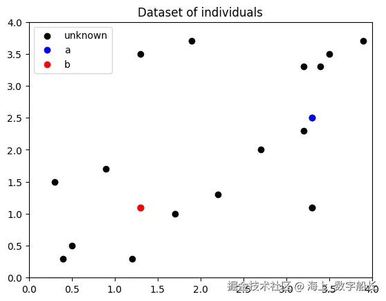

🔑 关键步骤：知识库的定义与核心规则解析

知识库 <math xmlns="http://www.w3.org/1998/Math/MathML"> K \mathcal{K} </math>K 本质上是：

你希望模型学会的全部先验知识，用一阶逻辑公式编码成的、模型必须遵守的约束集合。

它不是存储数据的数据库，而是给模型定的"标准答案 + 通用行为准则"。所有公式合起来，就是你想让模型掌握的完整知识体系。

对于该最近邻分类的例子来说，目前已经知道了两个已分类的点 point_a、point_b。以这两个点作为分类的基准点，在 points 中，对任意两个点 <math xmlns="http://www.w3.org/1998/Math/MathML"> x 1 x_1 </math>x1、 <math xmlns="http://www.w3.org/1998/Math/MathML"> x 2 x_2 </math>x2 以及任意标签 <math xmlns="http://www.w3.org/1998/Math/MathML"> l l </math>l，只要两个点足够相似，它们的分类结果就必须完全一致。最终，与点 point_a、point_b 相似的对应点，他们的标签会逐渐分类到 <math xmlns="http://www.w3.org/1998/Math/MathML"> A A </math>A、 <math xmlns="http://www.w3.org/1998/Math/MathML"> B B </math>B 两类。

首先，我们需要定义一个隶属谓词 <math xmlns="http://www.w3.org/1998/Math/MathML"> C ( x , l ) C(x,l) </math>C(x,l)，其中 <math xmlns="http://www.w3.org/1998/Math/MathML"> x x </math>x 是一个个体（点）， <math xmlns="http://www.w3.org/1998/Math/MathML"> l l </math>l 是一个 one-hot 标签，表示两个类别之一（10 表示类别 <math xmlns="http://www.w3.org/1998/Math/MathML"> A A </math>A，01 表示类别 <math xmlns="http://www.w3.org/1998/Math/MathML"> B B </math>B）。 <math xmlns="http://www.w3.org/1998/Math/MathML"> C C </math>C 通过一个简单的 MLP（多层感知器）进行逼近。最后一层计算每个类别的概率，使用 softmax 激活函数，确保类别是互斥的。

我们通过以下规则定义知识库 <math xmlns="http://www.w3.org/1998/Math/MathML"> K \mathcal{K} </math>K：
<math xmlns="http://www.w3.org/1998/Math/MathML" display="block"> C ( a , l a ) C ( b , l b ) ∀ x 1 , x 2 , l ( S i m ( x 1 , x 2 ) → ( C ( x 1 , l ) ↔ C ( x 2 , l ) ) ) \begin{aligned} & C(a,l_a) \ & C(b,l_b) \ & \forall x_1,x_2,l\ \big(\mathrm{Sim}(x_1,x_2) \rightarrow \big(C(x_1,l)\leftrightarrow C(x_2,l)\big)\big) \end{aligned} </math>C(a,la) C(b,lb) ∀x1,x2,l (Sim(x1,x2)→(C(x1,l)↔C(x2,l)))

其中：

<math xmlns="http://www.w3.org/1998/Math/MathML"> a a </math>a 和 <math xmlns="http://www.w3.org/1998/Math/MathML"> b b </math>b 是两个已分类的个体；
<math xmlns="http://www.w3.org/1998/Math/MathML"> x 1 x_1 </math>x1 和 <math xmlns="http://www.w3.org/1998/Math/MathML"> x 2 x_2 </math>x2 是变量，表示所有个体；
<math xmlns="http://www.w3.org/1998/Math/MathML"> l a l_a </math>la 和 <math xmlns="http://www.w3.org/1998/Math/MathML"> l b l_b </math>lb 是类别 <math xmlns="http://www.w3.org/1998/Math/MathML"> A A </math>A 和 <math xmlns="http://www.w3.org/1998/Math/MathML"> B B </math>B 的 one-hot 标签；
<math xmlns="http://www.w3.org/1998/Math/MathML"> l l </math>l 是一个变量，表示标签；
<math xmlns="http://www.w3.org/1998/Math/MathML"> S i m \mathrm{Sim} </math>Sim 是一个度量两个点相似度的谓词，定义为：

<math xmlns="http://www.w3.org/1998/Math/MathML" display="block"> G ( S i m ) : u ⃗ , v ⃗ ↦ exp ⁡ ( − ∣ u ⃗ − v ⃗ ∣ 2 ) \mathcal{G}(\mathrm{Sim}):\vec{u},\vec{v}\mapsto \exp(-|\vec{u}-\vec{v} |^2) </math>G(Sim):u ,v ↦exp(−∣u −v ∣2)

整个知识库 <math xmlns="http://www.w3.org/1998/Math/MathML"> K \mathcal{K} </math>K 里，唯一可学习、可调整的对象只有谓词 <math xmlns="http://www.w3.org/1998/Math/MathML"> C C </math>C； <math xmlns="http://www.w3.org/1998/Math/MathML"> K \mathcal{K} </math>K 的整体满足度由 <math xmlns="http://www.w3.org/1998/Math/MathML"> C C </math>C 的参数决定。

因此，目标是学习谓词 <math xmlns="http://www.w3.org/1998/Math/MathML"> C C </math>C 来最大化 <math xmlns="http://www.w3.org/1998/Math/MathML"> K \mathcal{K} </math>K 的满足度。也就是说：

训练分类器 <math xmlns="http://www.w3.org/1998/Math/MathML"> C C </math>C，让它尽可能满足我们设定的所有逻辑规则。🎯

🧩 <math xmlns="http://www.w3.org/1998/Math/MathML"> K \mathcal{K} </math>K 中包含的两类规则

第一类：事实公理（确定的、已知的标注知识）

对应公式里的前两条：
<math xmlns="http://www.w3.org/1998/Math/MathML" display="block"> C ( a , l a ) C(a,l_a) </math>C(a,la)
<math xmlns="http://www.w3.org/1998/Math/MathML" display="block"> C ( b , l b ) C(b,l_b) </math>C(b,lb)

含义：这是你给模型的板上钉钉的标注事实，没有任何模糊空间。
- <math xmlns="http://www.w3.org/1998/Math/MathML"> C ( a , l a ) C(a,l_a) </math>C(a,la)：个体 <math xmlns="http://www.w3.org/1998/Math/MathML"> a a </math>a 属于类别 <math xmlns="http://www.w3.org/1998/Math/MathML"> A A </math>A
- <math xmlns="http://www.w3.org/1998/Math/MathML"> C ( b , l b ) C(b,l_b) </math>C(b,lb)：个体 <math xmlns="http://www.w3.org/1998/Math/MathML"> b b </math>b 属于类别 <math xmlns="http://www.w3.org/1998/Math/MathML"> B B </math>B
作用：给模型锚定分类的"基准点"，是模型学习的起点，模型必须优先满足这两条，让它们的真值尽可能接近 1。

第二类：规则公理（通用的、泛化的逻辑规律）

对应第三条全称量化公式：
<math xmlns="http://www.w3.org/1998/Math/MathML" display="block"> ∀ x 1 , x 2 , l ( S i m ( x 1 , x 2 ) → ( C ( x 1 , l ) ↔ C ( x 2 , l ) ) ) \forall x_1,x_2,l\ \big(\mathrm{Sim}(x_1,x_2) \rightarrow \big(C(x_1,l)\leftrightarrow C(x_2,l)\big)\big) </math>∀x1,x2,l (Sim(x1,x2)→(C(x1,l)↔C(x2,l)))

含义：这是你给模型的通用归纳偏置，是不局限于特定样本、所有个体都必须遵守的核心规律。
大白话翻译：对任意两个点 <math xmlns="http://www.w3.org/1998/Math/MathML"> x 1 x_1 </math>x1、 <math xmlns="http://www.w3.org/1998/Math/MathML"> x 2 x_2 </math>x2，任意标签 <math xmlns="http://www.w3.org/1998/Math/MathML"> l l </math>l，只要两个点足够相似，它们的分类结果就必须完全一致。
作用：这是模型能够实现泛化的核心。你只给了 2 个标注样本，却可以靠这条规则，让模型对所有未见过的新样本做分类。🚀

🌟 该知识库 <math xmlns="http://www.w3.org/1998/Math/MathML"> K \mathcal{K} </math>K 的两个关键特点

它是可计算真值的封闭公式集合：所有公式都没有自由变量（要么针对确定的常量 <math xmlns="http://www.w3.org/1998/Math/MathML"> a / b a/b </math>a/b，要么所有变量都被全称量化 <math xmlns="http://www.w3.org/1998/Math/MathML"> ∀ \forall </math>∀ 约束），每一条都能算出一个 <math xmlns="http://www.w3.org/1998/Math/MathML"> [ 0 , 1 ] [0,1] </math>[0,1] 之间的真值。真值越接近 1，代表这条知识被模型满足的程度越高。
它是模型的优化目标本身：模型训练的唯一目标，就是让自己的行为（谓词 <math xmlns="http://www.w3.org/1998/Math/MathML"> C C </math>C 的输出）尽可能符合 <math xmlns="http://www.w3.org/1998/Math/MathML"> K \mathcal{K} </math>K 里的所有公式。

如果 <math xmlns="http://www.w3.org/1998/Math/MathML"> θ \theta </math>θ 表示可训练参数集，则参数集的训练目标为：
<math xmlns="http://www.w3.org/1998/Math/MathML" display="block"> θ ∗ = a r g m a x ∗ θ ∈ Θ S a t A g g ∗ ϕ ∈ K G θ ( ϕ ) \begin{aligned} \theta^\ast = \mathrm{argmax}*{\theta\in\Theta}\ \mathrm{SatAgg}*{\phi\in\mathcal{K}} \ \mathcal{G}_{\theta}(\phi) \end{aligned} </math>θ∗=argmax∗θ∈Θ SatAgg∗ϕ∈K Gθ(ϕ)

其中 <math xmlns="http://www.w3.org/1998/Math/MathML"> S a t A g g \mathrm{SatAgg} </math>SatAgg 是一个聚合 <math xmlns="http://www.w3.org/1998/Math/MathML"> K \mathcal{K} </math>K 中公式真值的运算符（如果有多个公式），默认用 pMeanError 实现 SatAgg。

💻 代码实现：训练循环搭建

为了在 LTN 中定义知识库，我们首先需要定义我们的谓词、变量和常量。在下面，谓词、变量和常量的名称与上述问题表述中的名称相同。

python 复制代码

# 谓词 C
class ModelC(torch.nn.Module):
    def __init__(self):
        super(ModelC, self).__init__()
        self.elu = torch.nn.ELU()
        self.softmax = torch.nn.Softmax(dim=1)
        self.dense1 = torch.nn.Linear(2, 5)
        self.dense2 = torch.nn.Linear(5, 5)
        self.dense3 = torch.nn.Linear(5, 2)

    def forward(self, x, l):
        """x: point, l: one-hot label"""
        x = self.elu(self.dense1(x))
        x = self.elu(self.dense2(x))
        prob = self.softmax(self.dense3(x))
        return torch.sum(prob * l, dim=1)

C = ltn.Predicate(ModelC().to(device))

# 代表相似程度的谓词
Sim = ltn.Predicate(func=lambda u, v: torch.exp(-1. * torch.sqrt(torch.sum(torch.square(u - v), dim=1))))

# 变量与常量
x1 = ltn.Variable("x1", torch.tensor(points))
x2 = ltn.Variable("x2", torch.tensor(points))
a = ltn.Constant(torch.tensor([3.3, 2.5]).to(device))
b = ltn.Constant(torch.tensor([1.3, 1.1]).to(device))
l_a = ltn.Constant(torch.tensor([1, 0]))
l_b = ltn.Constant(torch.tensor([0, 1]))
l = ltn.Variable("l", torch.tensor([[1, 0], [0, 1]]))

接下来，我们绘制数据集中每个点与点 <math xmlns="http://www.w3.org/1998/Math/MathML"> a a </math>a 的相似度。相似度越低，连接点的线条越细。

python 复制代码

similarities_to_a = Sim(x1, a).value
fig, ax = plt.subplots()
ax.set_xlim(0, 4)
ax.set_ylim(0, 4)
ax.scatter(points[:,0], points[:,1], color="black")
ax.scatter(a.value[0].cpu().numpy(), a.value[1].cpu().numpy(), color="blue")
ax.set_title("Illustrating the similarities of each point to a")
for i, sim_to_a in enumerate(similarities_to_a):
    plt.plot([points[i,0], a.value[0].cpu().numpy()], [points[i,1],a.value[1].cpu().numpy()], alpha=float(sim_to_a), color="blue")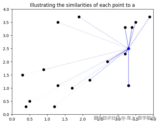

🧱 核心代码 1：谓词、变量、常量的定义

联结词使用稳定"乘积配置"。

等价运算符 <math xmlns="http://www.w3.org/1998/Math/MathML"> p ↔ q p \leftrightarrow q </math>p↔q 在 LTN 中实现为：
<math xmlns="http://www.w3.org/1998/Math/MathML" display="block"> ( p → q ) ∧ ( q → p ) (p \rightarrow q) \land (q \rightarrow p) </math>(p→q)∧(q→p)

它使用一个联结词运算符和一个蕴涵运算符。该运算符可以通过 ltn.fuzzy_ops.Equiv 访问。

python 复制代码

Not = ltn.Connective(ltn.fuzzy_ops.NotStandard())
And = ltn.Connective(ltn.fuzzy_ops.AndProd())
Or = ltn.Connective(ltn.fuzzy_ops.OrProbSum())
Implies = ltn.Connective(ltn.fuzzy_ops.ImpliesReichenbach())
Equiv = ltn.Connective(ltn.fuzzy_ops.Equiv(ltn.fuzzy_ops.AndProd(), ltn.fuzzy_ops.ImpliesReichenbach()))
Forall = ltn.Quantifier(ltn.fuzzy_ops.AggregPMeanError(p=2), quantifier="f")
Exists = ltn.Quantifier(ltn.fuzzy_ops.AggregPMean(p=6), quantifier="e")

现在我们已经定义了谓词、变量和常量，我们可以开始定义知识库。

🧮 核心代码 2：知识库与 SatAgg 运算符实现

如果在 <math xmlns="http://www.w3.org/1998/Math/MathML"> K \mathcal{K} </math>K 中有多个封闭公式，它们的真值需要进行聚合，这正是 <math xmlns="http://www.w3.org/1998/Math/MathML"> S a t A g g \mathrm{SatAgg} </math>SatAgg 运算符的作用。目前， <math xmlns="http://www.w3.org/1998/Math/MathML"> S a t A g g \mathrm{SatAgg} </math>SatAgg 仅支持封闭公式。封闭公式是没有自由变量的公式，即所有变量都是被量化的。

在 LTN 中， <math xmlns="http://www.w3.org/1998/Math/MathML"> S a t A g g \mathrm{SatAgg} </math>SatAgg 运算符可以通过 ltn.fuzzy_ops.SatAgg 访问。构造函数 SatAgg() 需要一个聚合运算符作为输入，该运算符将在运算符调用时用于聚合输入。具体而言，该运算符接受一个封闭公式的真值列表，并使用选定的聚合器返回这些值的聚合结果。

作为 SatAgg 聚合器，推荐使用受广义均值启发的运算符 pMeanError。

pMeanError 已经用于实现 <math xmlns="http://www.w3.org/1998/Math/MathML"> ∀ \forall </math>∀，在公式内部进行"变量级聚合"------把开公式里所有自由变量的可能取值聚合成一个标量真值，让开公式变成封闭公式。

构造函数 SatAgg() 使用 pMeanError 来定义运算符。在公式外部的"知识库级聚合"中，它再把知识库里多个已经是封闭公式的标量真值聚合成一个整体满足度。

超参数 <math xmlns="http://www.w3.org/1998/Math/MathML"> p p </math>p 再次提供了聚合公式的严格性灵活性：

<math xmlns="http://www.w3.org/1998/Math/MathML"> p = 1 p = 1 </math>p=1 对应于 mean
<math xmlns="http://www.w3.org/1998/Math/MathML"> p → + ∞ p \to +\infty </math>p→+∞ 对应于 min

接下来，我们定义 SatAgg 运算符和一个训练循环来学习我们的 LTN 模型。

如下代码所示，SatAgg 运算符接受知识库中的公式，并返回一个真值，这个真值被解释为整个知识库的满足度。由于希望最大化这个数值，因此需要通过梯度下降最小化 <math xmlns="http://www.w3.org/1998/Math/MathML"> 1 − S a t A g g 1 - \mathrm{SatAgg} </math>1−SatAgg。

在将公式传递给 SatAgg 运算符之前，不需要访问 value 属性。这是因为该运算符接受 LTNObject 实例作为输入。

在 LTN 的前向阶段，计算三个公式的真值；而在反向阶段，谓词 <math xmlns="http://www.w3.org/1998/Math/MathML"> C C </math>C 的权重会被调整，以最小化损失函数。

python 复制代码

# by default, SatAgg uses the pMeanError
sat_agg = ltn.fuzzy_ops.SatAgg()

# we need to learn the parameters of the predicate C
optimizer = torch.optim.Adam(C.parameters(), lr=0.001)

for epoch in range(2000):
    optimizer.zero_grad()
    loss = 1. - sat_agg(
        C(a, l_a),
        C(b, l_b),
        Forall([x1, x2, l], Implies(Sim(x1, x2), Equiv(C(x1, l), C(x2, l))))
    )
    loss.backward()
    optimizer.step()
    if epoch%200 == 0:
        print("Epoch %d: Sat Level %.3f "%(epoch, 1 - loss.item()))
print("Training finished at Epoch %d with Sat Level %.3f" %(epoch, 1 - loss.item()))

text 复制代码

Epoch 0: Sat Level 0.536 
Epoch 200: Sat Level 0.767 
Epoch 400: Sat Level 0.948 
Epoch 600: Sat Level 0.953 
Epoch 800: Sat Level 0.954 
Epoch 1000: Sat Level 0.955 
Epoch 1200: Sat Level 0.955 
Epoch 1400: Sat Level 0.955 
Epoch 1600: Sat Level 0.955 
Epoch 1800: Sat Level 0.955 
Training finished at Epoch 1999 with Sat Level 0.955

经过几个训练轮次后，系统已经学会根据知识库的规则识别接近点 <math xmlns="http://www.w3.org/1998/Math/MathML"> a a </math>a 或 <math xmlns="http://www.w3.org/1998/Math/MathML"> b b </math>b 的样本，并分别将其分类为类别 <math xmlns="http://www.w3.org/1998/Math/MathML"> A A </math>A 或 <math xmlns="http://www.w3.org/1998/Math/MathML"> B B </math>B。✅

接下来，我们绘制一个图，展示我们的 LTN 如何通过将知识库的满足度作为目标来学习分类数据点。当谓词 <math xmlns="http://www.w3.org/1998/Math/MathML"> C C </math>C 的满足度较高时，颜色越亮。在左侧，我们看到 <math xmlns="http://www.w3.org/1998/Math/MathML"> C C </math>C 正确地分类了类别 <math xmlns="http://www.w3.org/1998/Math/MathML"> A A </math>A 的点；在右侧，我们看到它正确地分类了类别 <math xmlns="http://www.w3.org/1998/Math/MathML"> B B </math>B 的点。

python 复制代码

fig = plt.figure(figsize=(10, 3))
fig.add_subplot(1, 2, 1)
plt.scatter(x1.value[:, 0].cpu().numpy(), x1.value[:, 1].cpu().numpy(), c=C(x1, l_a).value.detach().cpu().numpy(), vmin=0, vmax=1)
plt.title("C(x,l_a)")
plt.colorbar()
fig.add_subplot(1, 2, 2)
plt.scatter(x1.value[:, 0].cpu().numpy(), x1.value[:, 1].cpu().numpy(), c=C(x1, l_b).value.detach().cpu().numpy(), vmin=0, vmax=1)
plt.title("C(x,l_b)")
plt.colorbar()
plt.show()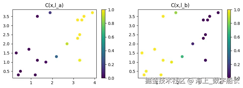

❓Q1：SatAgg 运算符的公式是什么？

⚡ 进阶：批次训练优化 LTN 学习效率

通过批次进行变量的构建

通常，在大多数学习任务中，我们使用数据批次来提高学习效率。在 LTN 中，使用数据批次非常简单，只需在每个训练步骤中使用不同的值来构建变量即可。

在 PyTorch 中，这些值通常通过 DataLoader 返回。下面用一个更大的数据集（10000 个点）来看同样的例子，这个数据集需要划分为小批次。数据集是随机生成的，点 <math xmlns="http://www.w3.org/1998/Math/MathML"> a a </math>a 和点 <math xmlns="http://www.w3.org/1998/Math/MathML"> b b </math>b 被选取的方式使得它们之间有足够的距离。

python 复制代码

r1 = 0
r2 = 4
points = (r1 - r2) * torch.rand((10000, 2)) + r2
points[-1] = torch.tensor([3., 3.])
points[-2] = torch.tensor([1., 1.])
points_a = torch.tensor([3., 3.])
points_b = torch.tensor([1., 1.])
a = ltn.Constant(torch.tensor([3., 3.]))
b = ltn.Constant(torch.tensor([1., 1.]))

fig, ax = plt.subplots()
ax.set_xlim(0, 4)
ax.set_ylim(0, 4)
ax.scatter(points[:,0], points[:,1], color="black", label="unknown")
ax.scatter(point_a[0], point_a[1], color="blue", label="a")
ax.scatter(point_b[0], point_b[1], color="red", label="b")
ax.set_title("Dataset of individuals")
plt.legend()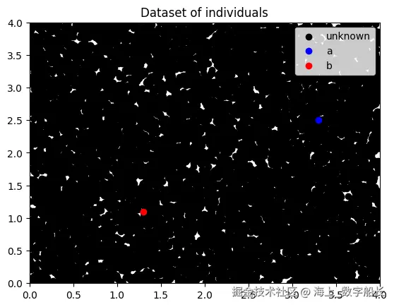

接下来，我们定义一个数据加载器 DataLoader，它接受整个数据集作为输入，并返回从数据集中获取的数据点批次。你可以决定批次大小以及是否对数据进行洗牌。

然后，如前所述，只需添加一些代码来遍历批次，并用批次中包含的新数据点构建变量。

python 复制代码

# we define C again to re-initialize its weights
C = ltn.Predicate(ModelC().to(device))

# data loader which creates the batches
class DataLoader:
    def __init__(self,
                 dataset,
                 batch_size=1,
                 shuffle=True):
        self.data = dataset
        self.batch_size = batch_size
        self.shuffle = shuffle

    def __len__(self):
        return int(np.ceil(self.data.shape[0] / self.batch_size))

    def __iter__(self):
        n = self.data.shape[0]
        idxlist = list(range(n))
        if self.shuffle:
            np.random.shuffle(idxlist)

        for _, start_idx in enumerate(range(0, n, self.batch_size)):
            end_idx = min(start_idx + self.batch_size, n)
            batch_points = self.data[idxlist[start_idx:end_idx]]

            yield batch_points

train_loader = DataLoader(points, 512)

# by default, SatAgg uses the pMeanError
sat_agg = ltn.fuzzy_ops.SatAgg()

# 需要学习的是谓词C的参数
optimizer = torch.optim.Adam(C.parameters(), lr=0.001)

for epoch in range(100):
    for (batch_idx, (batch_points)) in enumerate(train_loader):
        x1 = ltn.Variable("x1", batch_points)
        x2 = ltn.Variable("x2", batch_points)
        optimizer.zero_grad()
        loss = 1. - sat_agg(
            C(a, l_a),
            C(b, l_b),
            Forall([x1, x2, l], Implies(Sim(x1, x2), Equiv(C(x1, l), C(x2, l))))
        )
        loss.backward()
        optimizer.step()
    if epoch%10 == 0:
        print("Epoch %d: Sat Level %.3f "%(epoch, 1 - loss.item()))

print("Training finished at Epoch %d with Sat Level %.3f" %(epoch, 1 - loss.item()))

text 复制代码

Epoch 0: Sat Level 0.618 
Epoch 10: Sat Level 0.833 
Epoch 20: Sat Level 0.944 
Epoch 30: Sat Level 0.944 
Epoch 40: Sat Level 0.947 
Epoch 50: Sat Level 0.947 
Epoch 60: Sat Level 0.948 
Epoch 70: Sat Level 0.947 
Epoch 80: Sat Level 0.947 
Epoch 90: Sat Level 0.944 
Training finished at Epoch 99 with Sat Level 0.949

可以观察到，在 20 个训练轮次后，LTN 已经学会了正确地分类示例。📈

如图所示，LTN 已经学会了如何正确地分类数据点。同时，我们还可以观察到中间有一些点更难以分类。因为它们与点 <math xmlns="http://www.w3.org/1998/Math/MathML"> a a </math>a 和点 <math xmlns="http://www.w3.org/1998/Math/MathML"> b b </math>b 的距离相似，LTN 不知道应该为它们分配哪个正确的类别。

python 复制代码

x1 = ltn.Variable("x1", points)
x2 = ltn.Variable("x2", points)
fig = plt.figure(figsize=(10, 3))
fig.add_subplot(1, 2, 1)
plt.scatter(x1.value[:, 0].cpu().numpy(), x1.value[:, 1].cpu().numpy(), c=C(x1, l_a).value.detach().cpu().numpy(), vmin=0, vmax=1)
plt.title("C(x,l_a)")
plt.colorbar()
fig.add_subplot(1, 2, 2)
plt.scatter(x1.value[:, 0].cpu().numpy(), x1.value[:, 1].cpu().numpy(), c=C(x1, l_b).value.detach().cpu().numpy(), vmin=0, vmax=1)
plt.title("C(x,l_b)")
plt.colorbar()
plt.show();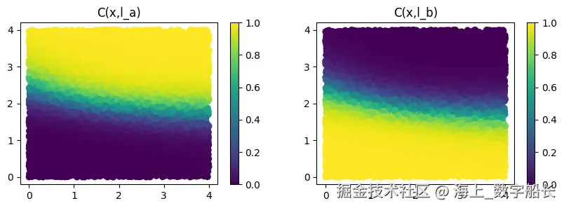

📝 总结与反思

本篇内容通过简单的最近邻分类示例，讲解了逻辑张量网络中如何构建包含逻辑、规则和先验的知识库，以及在学习过程中，模型是如何遵循知识库中的逻辑、规则和先验完成训练的。

后面的博文中，我们会使用 LTN 来实现更多基础的机器学习任务，并将 LTN 这类神经符号方法的理论和代码实现与传统神经网络的理论和代码实现进行对比，分析它们各自的优势与特点。🌱