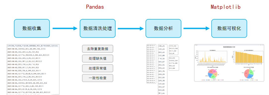
1.数据分析:从一堆看似杂乱的数据中,通过数据清洗、分析、可视化等手段,找出有价值的信息和结论,从而帮我们解决实际的问题(如:用户订单数据的分析、电影榜单数据分析、学校学生成绩分析等)。
2.环境准备
(1) Jupyter Notebook:是一个基于Web网页的、交互式的编程笔记本,让你可以把代码、运行结果、图表和笔记全部都放在一个文件里(在数据分析、机器学习、教学和科研等领域的数据实验室)
(2)Pandas:是一个功能强大的结构化数据分析的工具集,底层是基于Numpy构建的,无论是在数据分析领域、还是大数据开发场景中都有显著的优势。
核心:DataFrame(类似表格)、Series(类似表格中的一列)
PyCharm安装:pip install pandas==2.3
什么是DataFrame,什么是Series?
DataFrame是一个表格型的数据结构,就像一张Excel表格,有行有列;
Series是一列数据,就像DataFrame中的单独一列;
测试:
python
import pandas as pd

df1 = pd.DataFrame([
    {'姓名': '张三', '语文': 85, '数学': 92, '英语': 78},
    {'姓名': '李四', '语文': 78, '数学': 88, '英语': 95},
    {'姓名': '王五', '语文': 92, '数学': 96, '英语': 89},
    {'姓名': '赵六', '语文': 85, '数学': 90, '英语': 90},
    {'姓名': '孙七', '语文': 72, '数学': 59, '英语': 66},
    {'姓名': '周八', '语文': 80, '数学': 76, '英语': 68},
    {'姓名': '吴九', '语文': 85, '数学': 85, '英语': 85},
    {'姓名': '郑十', '语文': 57, '数学': 68, '英语': 49}])
print(f"最高分: {df1['语文'].max()}, 最低分: {df1['语文'].min()}, 平均分: {df1['语文'].mean()}")
print(f"最高分: {df1['数学'].max()}, 最低分: {df1['数学'].min()}, 平均分: {df1['数学'].mean()}")
print(f"最高分: {df1['英语'].max()}, 最低分: {df1['英语'].min()}, 平均分: {df1['英语'].mean()}")
最高分: 92, 最低分: 57, 平均分: 79.25
最高分: 96, 最低分: 59, 平均分: 81.75
最高分: 95, 最低分: 49, 平均分: 77.5
- 构建DataFrame的方式有很多,主要方式如下:
python
df1 = pd.DataFrame(
    {'姓名': '张三', '语文': 85, '数学': 92, '英语': 78},
    {'姓名': '李四', '语文': 78, '数学': 88, '英语': 95},
    {'姓名': '王五', '语文': 92, '数学': 96, '英语': 89})
df1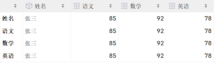
python
df2 = pd.DataFrame({
    '姓名': ['张三', '李四', '王五'],
    '语文': [85, 78, 92],
    '数学': [92, 88, 96],
    '英语': [78, 95, 89]})
df2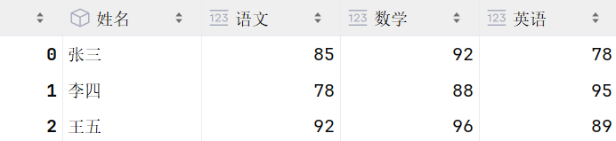
python
df3 = pd.DataFrame([
    ('张三', 85, 92, 78),
    ('李四', 78, 88, 95),
    ('王五', 92, 96, 89)
    ], columns=['姓名', '语文', '数学', '英语'])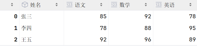
python
df4 = pd.DataFrame([
    ['张三', 85, 92, 78],
    ['李四', 78, 88, 95],
    ['王五', 92, 96, 89]
    ], columns=['姓名', '语文', '数学', '英语'], index=['a', 'b', 'c'])
df4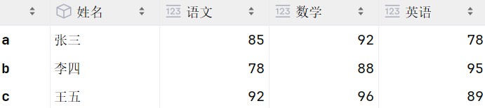
- 构建Series的方式有很多,主要方式如下:
python
s1 = pd.Series([10, 20, 30, 40, 50])

s2 = pd.Series((10, 20, 30, 40, 50), index=['a', 'b', 'c', 'd', 'e'])

s3 = pd.Series({'a': 10, 'b': 20, 'c': 30, 'd': 40, 'e': 50})

s4 = df4['语文']

# Series 常见属性 - index , values, size , dtype , shape
s3.index.tolist()  # index : 索引
s3.values.tolist()  # values : 值
s3.size  # size : 元素个数
s3.dtype  # dtype : 数据类型
s3.shape  # shape : 维度(行, )
DataFrame、Series中的常见属性的作用?
xx.index:获取索引
xx.values:获取值
xx.dtype:获取数据类型
xx.size:获取数据个数
xx.shape:获取数据维度(行,列)
xx.columns:获取列名(DataFrame特有属性)
3)数据读取和写入
python
import pandas as pd

# 读取数据 --> read_csv
df = pd.read_csv('data/sales.csv', usecols=['订单号', '产品类别', '产品名称', '销售数量', '单价'])

# 数据处理
df['销售金额'] = df['销售数量'] * df['单价']

# 写入数据 --> to_csv --- index=False: 不写入索引列
df.to_csv('data/sales_01.csv', index=False)
4)数据查看
查看:head()、tail()、describe()、info()
选择列:df'列名' / df\['列名1', '列名2']
选择行:df.ilocstart:stop:step / df.locstart:stop:step
python
# 数据查看 --> head , tail , describe , info , shape , columns
df1 = pd.read_csv('data/sales.csv', usecols=['订单号', '产品类别', '产品名称', '销售数量', '单价'])

df1.head(10) # 显示前10行数据
df1.tail(10) # 显示最后10行数据
df1.describe() # 显示数据统计信息  数量,平均值,统计值,最小值,25%,50%,75%,最大值
df1.info() # 显示数据信息(列名, 非空计数, 数据类型等)
df1.shape # 显示数据行数和列数
df1.columns # 显示列名语法:df条件表达式
示例:dfdf\['单价' >= 100] / dfdf\['类别'.isin('..','..')]
python
# 数据选择
df2 = pd.read_csv('data/sales.csv', usecols=['订单号', '产品类别', '产品名称', '销售数量', '单价'], index_col='订单号')

# 1. 选择列
# 1.1 单列
df2['产品名称']
df2.产品名称

# 1.2 多列
df2[['产品名称', '单价']]
df2[['产品类别', '产品名称', '单价']]

# 2. 选择行 - iloc , loc
# 2.1 iloc ----> 基于行号选择行 (不包含结束位置) , 语法: df.iloc[start:stop:step]
df2.iloc[0:5:1]
df2.iloc[0:5]

# 2.2 loc ----> 基于行索引选择行 (包含结束位置) , 语法: df.loc[start:stop:step]
df2.loc[6805677496:5878551159:2]
python
df3 = pd.read_csv('data/sales.csv')

# 配置项, 展示所有的数据
# pd.set_option('display.max_rows', None)

# 数据过滤 ---> df[filter]
# 1. 获取 销售数量 >= 10 的订单数据
df3[df3['销售数量'] >= 10]

# 2. 获取产品类别为 食品 或 图书 的订单数据
df3[df3['产品类别'].isin(['食品', '图书'])]

# 3. 获取 单价在100-200之间 的订单数据 ---> 范围: between ---> 默认包含边界 (inclusive="left")
df3[df3['单价'].between(79, 199)]

# 4. 获取 销售数量 >= 8 , 并且 单价 >= 100 的订单数据 ----> 多条件(并且: & , 或者: |)
df3[(df3['销售数量'] >= 8) & (df3['单价'] >= 100)]

# 5. 获取 产品类别为 服装/食品 , 支付方式为 支付宝/微信支付 的订单数据
df3[(df3['产品类别'].isin(['服装', '食品'])) & (df3['支付方式'].isin(['支付宝', '微信支付']))]
5)数据清洗:是指发现并纠正数据中可识别的错误的过程,包括处理缺失值、重复值、异常值,统一数据格式,保证数据的一致性。
isnull():查看缺失值
dropna():删除缺失值所在行
dropna(axis=1):删除缺失值所在列
fillna('**'):填充缺失值
ffill():填充缺失值,填充上一行
bfill():填充缺失值,填充下一行
duplicated():查看重复值(所有的列的数据都重复)
drop_duplicates():删除重复值
df'xx' = df'xx'.abs():修复异常值,取绝对值
df'xxx'.str.replace('/', '-'):数据格式处理
python
import pandas as pd

pd.set_option('display.min_rows', 30) # 设置显示行数(默认10行)

# 1. 读取数据
df = pd.read_csv('data/sales.csv')

# 2. 数据清洗
# 2.1 缺失值处理
df.isnull() # 查看缺失值

# 2.1.1 删除缺失值
df.dropna() # 删除缺失值所在行
df = df.dropna(axis=1) # 删除缺失值所在列
df

# 2.1.2 填充缺失值
df.fillna('--') # 填充缺失值
df.ffill() # 填充缺失值, 填充上一行数据
df.bfill() # 填充缺失值, 填充下一行数据
python
# 2.2 重复值处理
# 2.2.1 查看重复值
df.duplicated() # 查看重复值(所有的列的数据都重复)
df.duplicated(subset=['订单号']) # 查看重复值(指定列的数据重复)

# 2.2.2 删除重复值
df.drop_duplicates(subset=['订单号']) # keep='last' 保留重复值最后一行; keep='first' 保留重复值第一行;
python
# 2.3 异常值处理
# 2.3.1 查看异常值
df[df['单价'] <0]

# 2.3.2 删除异常值
df.drop(df[df['单价'] <0].index)

# 2.3.3 修复异常值
df['单价'] = df['单价'].abs() # 绝对值
df

# 2.4 数据格式处理
df['订单日期'] = df['订单日期'].str.replace('/', '-')
df
6)数据排序:在进行数据排序时,有两种排序方式,分别是:升序和降序。而基于Pandas进行数据排序时,是可以按照多个列进行排序的。
多列排序:进行多个列排序时,会先按照第一列进行排序,第一列的值相同时,才会按照第二列进行排序。
df.sort_values('销售数量', ascending=False):根据销售数量 倒序排序
df.sort_values('销售数量', '订单日期', ascending=True, False):根据销售数量升序排序,数量相同,再根据订单日期降序排序
df.sort_values('销售数量', '订单日期', ascending=False) :根据销售数量,订单日期降序排序
python
import pandas as pd

# 1. 读取数据
df = pd.read_csv('data/sales.csv', nrows=10)

# 2. 排序
# 2.1 根据 销售数量 倒序排序
df.sort_values('销售数量', ascending=False)

# 2.2 根据 单价 升序排序
df.sort_values('单价', ascending=True)
df.sort_values('单价')

# 2.3 根据 单价 升序排序, 价格一样, 再根据 销售数量 倒序排序
df.sort_values(['单价', '销售数量'], ascending=[True, False])
df.sort_values(['单价', '销售数量'], ascending=True)
7)数据分组:分组操作就是把数据按照某个特征分成不同的组,然后对每个组分别进行统计计算。
df.groupby('产品类别')'销售额'.sum():根据产品类别分组,统计各个类别的销售数量之和
df.groupby('产品类别')'销售额'.max():根据产品类别分组,统计各个类别的最高商品单价
df.groupby('产品类别')'销售额'.min():根据产品类别分组,统计各个类别的最低商品单价
df.groupby('产品类别')'销售额'.count():根据产品类别分组,统计各个类别的订单数量
df.groupby('产品类别')'销售额'.mean():根据产品类别分组,统计各个类别的平均商品
df.groupby('产品类别')'销售额'.agg('sum', 'max', 'min'):根据产品类别分组,统计各个类别的商品的销售数量之和、最大数量、最小数量
df.groupby('产品类别').agg('销售数量':'sum', '销售金额':'sum', '单价':'mean') :根据产品类别分组,统计各个类别的商品的销售数量之和,销售金额之和,平均单价
python
df = pd.read_csv('data/sales.csv', nrows=20)
df['销售金额'] = df['单价'] * df['销售数量']

# 3. 分组
# 3.1 根据 产品类别 分组, 统计各个类别的 订单数量 - count
df.groupby('产品类别')['订单号'].count()

# 3.2 根据 产品类别 分组, 统计各个类别的 销售数量 之和 - sum
df.groupby('产品类别')['销售数量'].sum()

# 3.3 根据 产品类别 分组, 统计各个类别的 销售金额 之和 - sum
df.groupby('产品类别')['销售金额'].sum()

# 3.4 根据 产品类别 分组, 统计各个类别的最低商品 单价 - min
df.groupby('产品类别')['单价'].min()

# 3.5 根据 产品类别 分组, 统计各个类别的最高商品 单价 - max
df.groupby('产品类别')['单价'].max()

# 3.6 根据 产品类别 分组, 统计各个类别的平均商品 单价 - mean
df.groupby('产品类别')['单价'].mean()

# 3.7 根据 产品类别 分组, 统计各个类别的商品的 平均单价、最高单价、最低单价 - agg
df.groupby('产品类别')['单价'].agg(['mean', 'max', 'min'])
df.groupby('产品类别').agg({'单价': ['mean', 'max', 'min']})

# 3.8 根据 产品类别 分组, 统计各个类别的商品的 销售数量 之和,销售金额 之和,平均 单价
df.groupby('产品类别').agg({'销售数量': 'sum', '销售金额': 'sum', '单价': 'mean'})
3.Matplotlib
Matplotlib是一个功能强大的数据可视化开源Python库,也是Python中使用的最多的图形绘图库,可以创建静态、动态、交互式的图表。
安装:pip install matplotlib
python
import matplotlib.pyplot as plt
import random

# 目标: 绘制折线图
x = [1, 2, 3, 4, 5, 6, 7, 8, 9, 10, 11, 12, 13, 14, 15, 16, 17, 18, 19, 20, 21, 22, 23, 24]
y = [1, 2, 3, 4, 5, 6, 7, 8, 9, 10, 11, 12, 13, 14, 15, 16, 17, 18, 19, 20, 21, 22, 23, 24]
y = [random.randint(10,15) for i in x]

plt.plot(x, y)# 折线图
plt.show() # 显示图表
python
import matplotlib.pyplot as plt
import random

# 展示中文
plt.rcParams['font.sans-serif'] = ['SimHei'] # 设置中文字体为黑体

x = [i for i in range(1, 25)]
y_bj = [random.randint(10,15) for i in x]
y_xa = [random.randint(13,18) for i in x]

plt.figure(figsize=(10, 5)) # 设置画布大小, 宽, 高
plt.plot(x, y_bj, label='北京') # 折线图 -> 如果没有画布, 会自动创建一个画布
plt.plot(x, y_xa, label='西安')

# 设置折线图的详细信息
plt.title('气温变化折线图', fontsize=15) # 标题
plt.xlabel('时间') # x轴标签
plt.ylabel('温度') # y轴标签
# plt.xticks(x[::2])
# plt.xticks(x[1::2])
plt.xticks(x) # x轴刻度
y_ticks = [i for i in range(5,21)]
plt.yticks(y_ticks) # y轴刻度
plt.grid(linestyle='--', alpha=0.3) # 显示网格
plt.legend(loc='upper right') # 显示图例

plt.show() # 显示图表
图表
python
from matplotlib.axes import Axes
import matplotlib.pyplot as plt

# 展示中文
plt.rcParams['font.sans-serif'] = ['SimHei'] # 设置中文字体为黑体

# 创建子图
# figure: 画布对象 ; axes: 子图数组(里面存放的是 Axes 类型的对象)
figure, axes = plt.subplots(nrows=1, ncols=2, figsize=(20,6), dpi=100) # nrows: 行 , ncols: 列

# 图一: 柱状图 (世界石油储备) - bar方法
countries = ['中国', '美国', '印度', '加拿大', '伊拉克', '沙特', '伊朗', '英国', '德国'] # 国家列表
values = [35, 23, 18, 21, 56, 78, 51, 12, 18]

axes1: Axes = axes[0]
axes1.bar(countries, values, width=0.6, color='g') # 柱状图 - width: 柱子宽度, color: 颜色
axes1.set_title('世界石油储备', fontsize=18) # 设置标题
axes1.set_xlabel('国家') # X轴标签
axes1.set_ylabel('石油储备(亿吨)') # Y轴标签
axes1.grid(linestyle='--', alpha=0.3) # 网格线


# 图二: 饼状图 (世界人口) --- > 擅长比例分析 -- pie 方法
countries2 = ['印度', '中国', '美国', '印尼', '巴基斯坦', '尼日利亚', '巴西', '俄罗斯', '其他']
values = [14.51, 14.09, 3.4, 2.83, 2.51, 2.33, 2.12, 1.44, 20]

axes2: Axes = axes[1]
axes2.pie(values, labels=countries2, autopct='%1.1f%%') # 饼状图
axes2.set_title('世界人口比例', fontsize=18) # 设置标题
axes2.legend(loc='lower center', ncol=5, bbox_to_anchor=(0.5, -0.08)) # 显示图例, ncol: 每行显示的个数, bbox_to_anchor: 图例位置(0.5 控制水平方位, -0.08 控制垂直方位)

# 保存图片
plt.savefig('data/01.png')

plt.show() # 展示图表
案列:TDB-TOP300电影榜单数据统计
python
from matplotlib.axes import Axes
import pandas as pd
import matplotlib.pyplot as plt
from pandas import Series

# 展示中文
plt.rcParams['font.sans-serif'] = ['SimHei']

# 创建子图
fig, axes = plt.subplots(nrows=2, ncols=2, figsize=(20, 12), dpi=100)
fig.suptitle('TMDB-TOP300电影榜单数据统计', fontsize=23, x=0.5, y=0.95) # 添加画布标题 - x=0.5 : X轴位置;  y=0.95 : Y轴位置
fig.subplots_adjust(hspace=0.4, wspace=0.2)  # 调整子图间距, hspace: 控制垂直间距,wspace: 控制水平间距

# 获取子图
axes1: Axes = axes[0][0]
axes2: Axes = axes[0][1]
axes3: Axes = axes[1][0]
axes4: Axes = axes[1][1]

# 加载数据
# int64 : 整型数字 (不支持空值);  Int64 : 整型数字 (支持空值); float64 : 浮点型数字 (支持空值);
data = pd.read_csv('data/movies.csv', usecols=['电影名','年份','上映时间','类型','时长','评分','语言'], dtype={'年份':'Int64'})


# 1. 需求一: 统计TOP300的电影中,每一年上映的电影数量的变化。(折线图)
# 1.1 缺失值、异常值处理
# data.isnull().sum()
data['年份'] = data['年份'].fillna(data['上映时间'].str[:4])

# 1.2 分组统计
year_count = data.groupby('年份')['年份'].count()

# 1.3 组装数据
# x轴数据
min_year = year_count.index.min()
max_year = year_count.index.max()
x = [i for i in range(min_year, max_year+1)]

# y轴数据
y = [int(year_count.get(i, 0)) for i in x]

# 1.4 绘制折线图
axes1.plot(x, y, color='green') # 折线图
axes1.set_title('每年电影数量变化折线图', fontsize=18) # 添加子图标题
axes1.set_xlabel('年份', fontsize=12)  # 添加X轴标签
axes1.set_ylabel('电影数量', fontsize=12) # 添加Y轴标签

axes1.set_xticks(x[::8]) # 设置X轴刻度间隔
y_ticks = [i for i in range(0,31,3)]
axes1.set_yticks(y_ticks) # 设置Y轴刻度间隔
axes1.grid(linestyle='--', alpha=0.5) # 添加网格线


# 2. 需求二: 统计对比不同语言的电影数量。(柱状图)
# 2.1 获取不同语言对应的电影数量
language_count = data.groupby('语言')['语言'].count().sort_values(ascending=False)

x_language = language_count.index.tolist()
y_language_count = language_count.values.tolist()

# 2.2 绘制柱状图
axes2.bar(x_language, y_language_count, color='green', width=0.7) # 柱状图
axes2.set_title('不同语言电影数量柱状图', fontsize=18) # 添加子图标题
axes2.set_xlabel('语言', fontsize=12) # 添加X轴标签
axes2.set_ylabel('电影数量', fontsize=12) # 添加Y轴标签
axes2.grid(linestyle='--', alpha=0.5) # 添加网格线
axes2.tick_params(axis='x', rotation=90) # 旋转X轴标签


# 3. 需求三: 统计对比不同类型电影数量 (柱状图)
# 3.1 获取不同类型对应的电影数量
type_count = {} # {'剧情': 5, '犯罪': 3}
for types in data['类型'].str.split(','): # [剧情,犯罪]
    for t in types: # 剧情
        if t in type_count:
            type_count[t] += 1
        else:
            type_count[t] = 1

x_types = list(type_count.keys()) # 类型列表
y_values = list(type_count.values()) # 数量列表

# 3.2 绘制柱状图
axes3.bar(x_types, y_values, color='green', width=0.7) # 柱状图
axes3.set_title('不同类型电影数量柱状图', fontsize=18) # 添加子图标题
axes3.set_xlabel('类型', fontsize=12) # 添加X轴标签
axes3.set_ylabel('电影数量', fontsize=12) # 添加Y轴标签
axes3.grid(linestyle='--', alpha=0.5) # 添加网格线
axes3.tick_params(axis='x', rotation=90) # 旋转X轴标签


# 4. 需求四: 统计不同评分电影数量占比 (饼状图)
# 4.1 获取不同评分对应的电影数量
score_count = data.groupby('评分')['评分'].count()

# 合并小数据(比例 < 2%) --> 其他
total = score_count.sum()
large_scores: Series = score_count.loc[score_count >= total*0.02] # 大数据 , 比例 >= 2%
small_scores: Series = score_count.loc[score_count < total*0.02] # 小数据 , 比例 < 2%

if small_scores.shape[0] > 0:
    large_scores['其他'] = small_scores.sum()

scores = large_scores.index.tolist() # 评分列表
scores_values = large_scores.values.tolist() # 数量列表

# 4.2 绘制饼状图
axes4.pie(scores_values, labels=scores, autopct='%1.1f%%', startangle=0, radius=1.2) # startangle 起始角度
axes4.set_title('不同评分电影数量占比饼状图', fontsize=18)
axes4.legend(loc='lower center', ncol=4, bbox_to_anchor=(0.5, -0.2))


# 5. 保存图片
plt.savefig('data/TMDB-TOP300.png')

plt.show() # 显示画布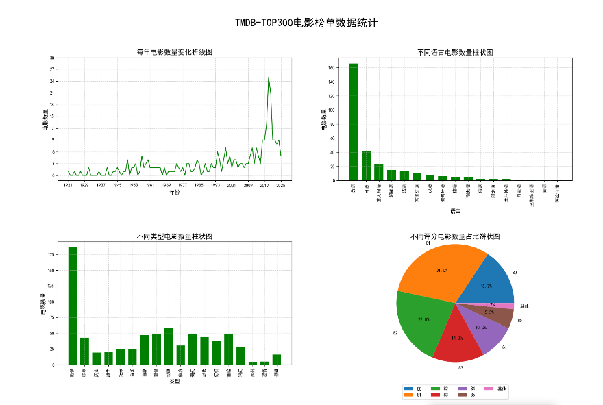
python文件
python
"""
TMDB-TOP300电影榜单数据统计
"""

import pandas as pd
import matplotlib.pyplot as plt
from matplotlib.axes import Axes
from pandas import Series

# 展示中文
plt.rcParams['font.sans-serif'] = ['SimHei']

def load_data():
    """
    加载电影数据
    """
    return pd.read_csv('data/movies.csv', usecols=['电影名','年份','上映时间','类型','时长','评分','语言'], dtype={'年份':'Int64'})

def create_subplots():
    """
    创建子图布局
    """
    fig, axes = plt.subplots(nrows=2, ncols=2, figsize=(20, 12), dpi=100)
    fig.suptitle('TMDB-TOP300电影榜单数据统计', fontsize=23, x=0.5, y=0.98)
    fig.subplots_adjust(hspace=0.5, wspace=0.2)

    axes1: Axes = axes[0][0]
    axes2: Axes = axes[0][1]
    axes3: Axes = axes[1][0]
    axes4: Axes = axes[1][1]

    return fig, axes, axes1, axes2, axes3, axes4

def process_year_data(data):
    """
    处理年份数据并生成折线图所需的数据
    """
    # 缺失值处理
    data['年份'] = data['年份'].fillna(data['上映时间'].str[:4])

    # 分组统计
    year_count = data.groupby('年份')['年份'].count()

    # 组装数据
    min_year = year_count.index.min()
    max_year = year_count.index.max()
    x = [i for i in range(min_year, max_year+1)]
    y = [int(year_count.get(i, 0)) for i in x]

    return x, y

def plot_year_trend(axes1, x, y):
    """
    绘制每年电影数量变化折线图
    """
    axes1.plot(x, y, color='green')
    axes1.set_title('每年电影数量变化折线图', fontsize=15)
    axes1.set_xlabel('年份', fontsize=12)
    axes1.set_ylabel('电影数量', fontsize=12)

    axes1.set_xticks(x[::8])
    y_ticks = [i for i in range(0,31,3)]
    axes1.set_yticks(y_ticks)
    axes1.grid(linestyle='--', alpha=0.5)

def process_language_data(data):
    """
    处理语言数据并生成柱状图所需的数据
    """
    language_count = data.groupby('语言')['语言'].count().sort_values(ascending=False)
    x_language = language_count.index.tolist()
    y_language_count = language_count.values.tolist()
    return x_language, y_language_count

def plot_language_bar(axes2, x_language, y_language_count):
    """
    绘制不同语言电影数量柱状图
    """
    axes2.bar(x_language, y_language_count, color='green', width=0.7)
    axes2.set_title('不同语言电影数量柱状图', fontsize=15)
    axes2.set_xlabel('语言', fontsize=12)
    axes2.set_ylabel('电影数量', fontsize=12)
    axes2.grid(linestyle='--', alpha=0.5)
    axes2.tick_params(axis='x', rotation=90)

def process_genre_data(data):
    """
    处理类型数据并生成柱状图所需的数据
    """
    type_count = {}
    for types in data['类型'].str.split(','):
        for t in types:
            if t in type_count:
                type_count[t] += 1
            else:
                type_count[t] = 1

    x_types = list(type_count.keys())
    y_values = list(type_count.values())
    return x_types, y_values

def plot_genre_bar(axes3, x_types, y_values):
    """
    绘制不同类型电影数量柱状图
    """
    axes3.bar(x_types, y_values, color='green', width=0.7)
    axes3.set_title('不同类型电影数量柱状图', fontsize=15)
    axes3.set_xlabel('类型', fontsize=12)
    axes3.set_ylabel('电影数量', fontsize=12)
    axes3.grid(linestyle='--', alpha=0.5)
    axes3.tick_params(axis='x', rotation=90)

def process_score_data(data):
    """
    处理评分数据并生成饼状图所需的数据
    """
    score_count = data.groupby('评分')['评分'].count()

    # 合并小数据(比例 < 2%) --> 其他
    total = score_count.sum()
    large_scores = score_count.loc[score_count >= total*0.02]
    small_scores = score_count.loc[score_count < total*0.02]

    if small_scores.shape[0] > 0:
        large_scores['其他'] = small_scores.sum()

    scores = large_scores.index.tolist()
    scores_values = large_scores.values.tolist()
    return scores, scores_values

def plot_score_pie(axes4, scores, scores_values):
    """
    绘制不同评分电影数量占比饼状图
    """
    axes4.pie(scores_values, labels=scores, autopct='%1.1f%%', startangle=0, radius=1.2)
    axes4.set_title('不同评分电影数量占比饼状图', fontsize=15)
    axes4.legend(loc='lower center', ncol=4, bbox_to_anchor=(0.5, -0.3))

def main():
    """
    主函数
    """
    # 加载数据
    data = load_data()

    # 创建子图
    fig, axes, axes1, axes2, axes3, axes4 = create_subplots()

    # 需求一:每年电影数量变化折线图
    x, y = process_year_data(data)
    plot_year_trend(axes1, x, y)

    # 需求二:不同语言电影数量柱状图
    x_language, y_language_count = process_language_data(data)
    plot_language_bar(axes2, x_language, y_language_count)

    # 需求三:不同类型电影数量柱状图
    x_types, y_values = process_genre_data(data)
    plot_genre_bar(axes3, x_types, y_values)

    # 需求四:不同评分电影数量占比饼状图
    scores, scores_values = process_score_data(data)
    plot_score_pie(axes4, scores, scores_values)

    # 保存图片
    plt.savefig('data/TMDB-TOP300.png')

    # 显示画布
    plt.show()

if __name__ == '__main__':
    main()