Day 6 编程实战：决策树与过拟合分析

Day 6 编程实战：决策树与过拟合分析

实战目标

1. 手动实现决策树（信息增益和基尼系数）
2. 理解不同分裂准则的差异
3. 可视化决策树结构
4. 观察不同max_depth下的过拟合现象
5. 使用剪枝参数控制过拟合

1. 导入必要的库

import numpy as np
import pandas as pd
import matplotlib.pyplot as plt
import seaborn as sns
from sklearn.datasets import make_classification, make_regression
from sklearn.model_selection import train_test_split, cross_val_score
from sklearn.tree import DecisionTreeClassifier, DecisionTreeRegressor, plot_tree, export_text
from sklearn.metrics import accuracy_score, classification_report, confusion_matrix
from sklearn.preprocessing import StandardScaler
import warnings
warnings.filterwarnings('ignore')

# 启用LaTeX渲染（如果系统安装了LaTeX）
plt.rcParams['text.usetex'] = False  # 设为False避免LaTeX依赖
# 设置中文显示
plt.rcParams['font.sans-serif'] = ['SimHei', 'Microsoft YaHei', 'DejaVu Sans']
plt.rcParams['axes.unicode_minus'] = False

2. 信息熵与基尼系数可视化

2.1 二分类下的熵和基尼系数

def entropy(p):
    """计算二分类熵"""
    p = np.clip(p, 1e-15, 1 - 1e-15)
    return -(p * np.log2(p) + (1 - p) * np.log2(1 - p))

def gini(p):
    """计算二分类基尼系数"""
    return 1 - p**2 - (1-p)**2

# 生成概率值
p = np.linspace(0, 1, 100)
entropy_values = entropy(p)
gini_values = gini(p)

# 绘图
plt.figure(figsize=(8, 3))

plt.subplot(1, 2, 1)
plt.plot(p, entropy_values, 'b-', linewidth=2, label='熵')
plt.plot(p, gini_values, 'r-', linewidth=2, label='基尼系数')
plt.xlabel('正类概率 p')
plt.ylabel('不纯度')
plt.title('二分类不纯度度量')
plt.legend()
plt.grid(True, alpha=0.3)
plt.axvline(x=0.5, color='k', linestyle='--', alpha=0.5)

plt.subplot(1, 2, 2)
plt.plot(p, entropy_values, 'b-', linewidth=2, label='熵', alpha=0.7)
plt.plot(p, gini_values, 'r-', linewidth=2, label='基尼系数', alpha=0.7)
plt.fill_between(p, entropy_values, gini_values, alpha=0.2)
plt.xlabel('正类概率 p')
plt.ylabel('不纯度')
plt.title('熵 vs 基尼系数对比')
plt.legend()
plt.grid(True, alpha=0.3)

plt.tight_layout()
plt.show()

print("观察结论:")
print("- 熵和基尼系数都是凸函数，形状相似")
print("- 基尼系数计算更快（无需对数）")
print("- 实际应用中两者效果相近")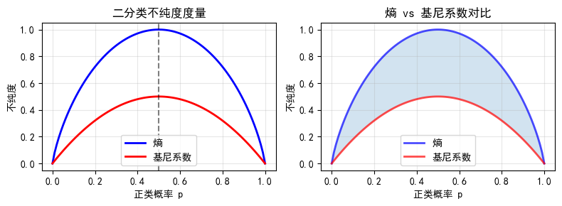

观察结论:
- 熵和基尼系数都是凸函数，形状相似
- 基尼系数计算更快（无需对数）
- 实际应用中两者效果相近

2.2 多分类下的熵

def multiclass_entropy(probabilities):
    """计算多分类熵"""
    probabilities = np.clip(probabilities, 1e-15, 1)
    return -np.sum(probabilities * np.log2(probabilities))

# 示例：三分类
classes = ['类A', '类B', '类C']
scenarios = [
    ([1.0, 0, 0], "完全纯（全部是类A）"),
    ([0.6, 0.3, 0.1], "偏斜分布"),
    ([0.34, 0.33, 0.33], "均匀分布")
]

print("多分类熵示例:")
print("-" * 50)
for probs, desc in scenarios:
    ent = multiclass_entropy(probs)
    print(f"{desc}: {probs} → 熵 = {ent:.4f}")

多分类熵示例:
--------------------------------------------------
完全纯（全部是类A）: [1.0, 0, 0] → 熵 = 0.0000
偏斜分布: [0.6, 0.3, 0.1] → 熵 = 1.2955
均匀分布: [0.34, 0.33, 0.33] → 熵 = 1.5848

3. 手动实现分类决策树

实现基尼系数和信息增益计算

class DecisionTreeManual:
    """手动实现决策树（简化版）"""
    
    def __init__(self, max_depth=None, min_samples_split=2, criterion='gini'):
        self.max_depth = max_depth
        self.min_samples_split = min_samples_split
        self.criterion = criterion  # 'gini' or 'entropy'
        self.tree = None
    
    def _gini(self, y):
        """计算基尼系数"""
        classes = np.unique(y)
        # 所有样本同一类：Gini = 0（最纯）
        if len(classes) == 1:
            return 0
        probs = [np.sum(y == c) / len(y) for c in classes]
        return 1 - np.sum([p**2 for p in probs])
    
    def _entropy(self, y):
        """计算熵"""
        classes = np.unique(y)
        # 所有样本同一类：熵 = 0（最纯）
        if len(classes) == 1:
            return 0
        probs = [np.sum(y == c) / len(y) for c in classes]
        return -np.sum([p * np.log2(p) for p in probs if p > 0])
    
    def _impurity(self, y):
        """计算不纯度"""
        if self.criterion == 'gini':
            return self._gini(y)
        else:
            return self._entropy(y)
    
    def _best_split(self, X, y):
        """找到最佳分裂特征和阈值"""
        best_gain = -1
        best_feature = None
        best_threshold = None
        
        n_samples, n_features = X.shape
        current_impurity = self._impurity(y)
        
        for feature in range(n_features):
            # 获取特征值并排序
            feature_values = X[:, feature]
            unique_values = np.unique(feature_values)
            
            # 尝试每个可能的分割点
            for threshold in unique_values:
                # 分割数据
                left_mask = feature_values <= threshold
                right_mask = feature_values > threshold
                
                if np.sum(left_mask) < self.min_samples_split or np.sum(right_mask) < self.min_samples_split:
                    continue
                
                # 计算加权不纯度
                left_impurity = self._impurity(y[left_mask])
                right_impurity = self._impurity(y[right_mask])
                n_left = np.sum(left_mask)
                n_right = np.sum(right_mask)
                
                weighted_impurity = (n_left / n_samples) * left_impurity + (n_right / n_samples) * right_impurity
                
                # 计算信息增益
                gain = current_impurity - weighted_impurity
                
                if gain > best_gain:
                    best_gain = gain
                    best_feature = feature
                    best_threshold = threshold
        
        return best_feature, best_threshold, best_gain
    
    def _build_tree(self, X, y, depth=0):
        """递归构建决策树"""
        n_samples, n_features = X.shape
        n_classes = len(np.unique(y))
        
        # 停止条件
        if (self.max_depth is not None and depth >= self.max_depth) or \
           n_samples < self.min_samples_split or \
           n_classes == 1:
            # 返回叶节点（多数类）
            unique, counts = np.unique(y, return_counts=True)
            return {'leaf': True, 'prediction': unique[np.argmax(counts)]}
        
        # 寻找最佳分裂
        feature, threshold, gain = self._best_split(X, y)
        
        if feature is None or gain <= 0:
            unique, counts = np.unique(y, return_counts=True)
            return {'leaf': True, 'prediction': unique[np.argmax(counts)]}
        
        # 分割数据
        left_mask = X[:, feature] <= threshold
        right_mask = X[:, feature] > threshold
        
        # 递归构建子树
        left_subtree = self._build_tree(X[left_mask], y[left_mask], depth + 1)
        right_subtree = self._build_tree(X[right_mask], y[right_mask], depth + 1)
        
        return {
            'leaf': False,
            'feature': feature,
            'threshold': threshold,
            'left': left_subtree,
            'right': right_subtree,
            'gain': gain
        }
    
    def fit(self, X, y):
        """训练决策树"""
        self.tree = self._build_tree(X, y)
        return self
    
    def _predict_single(self, x, node):
        """预测单个样本"""
        if node['leaf']:
            return node['prediction']
        
        if x[node['feature']] <= node['threshold']:
            return self._predict_single(x, node['left'])
        else:
            return self._predict_single(x, node['right'])
    
    def predict(self, X):
        """批量预测"""
        return np.array([self._predict_single(x, self.tree) for x in X])

# 测试手动实现
X_test_tree, y_test_tree = make_classification(n_samples=200, n_features=4, random_state=42)
X_train_t, X_test_t, y_train_t, y_test_t = train_test_split(X_test_tree, y_test_tree, test_size=0.3)

# 手动决策树
manual_tree = DecisionTreeManual(max_depth=3, criterion='gini')
manual_tree.fit(X_train_t, y_train_t)
manual_pred = manual_tree.predict(X_test_t)

# sklearn决策树
sklearn_tree = DecisionTreeClassifier(max_depth=3)
sklearn_tree.fit(X_train_t, y_train_t)
sklearn_pred = sklearn_tree.predict(X_test_t)

print(f"手动实现准确率: {accuracy_score(y_test_t, manual_pred):.4f}")
print(f"sklearn实现准确率: {accuracy_score(y_test_t, sklearn_pred):.4f}")

手动实现准确率: 0.9000
sklearn实现准确率: 0.9000

4. 决策树可视化

4.1 生成可解释的示例数据

# 生成简单的二分类数据（便于理解）
from sklearn.datasets import make_blobs

# 生成三个簇的数据
X_blob, y_blob = make_blobs(n_samples=300, centers=2, n_features=2, 
                            cluster_std=1.5, random_state=42)

# 可视化数据
plt.figure(figsize=(6, 4))
plt.scatter(X_blob[y_blob==0, 0], X_blob[y_blob==0, 1], c='blue', label='类别0', alpha=0.6)
plt.scatter(X_blob[y_blob==1, 0], X_blob[y_blob==1, 1], c='red', label='类别1', alpha=0.6)
plt.xlabel('特征1')
plt.ylabel('特征2')
plt.title('示例数据分布')
plt.legend()
plt.grid(True, alpha=0.3)
plt.show()

# 训练决策树
tree_viz = DecisionTreeClassifier(max_depth=3, random_state=42)
tree_viz.fit(X_blob, y_blob)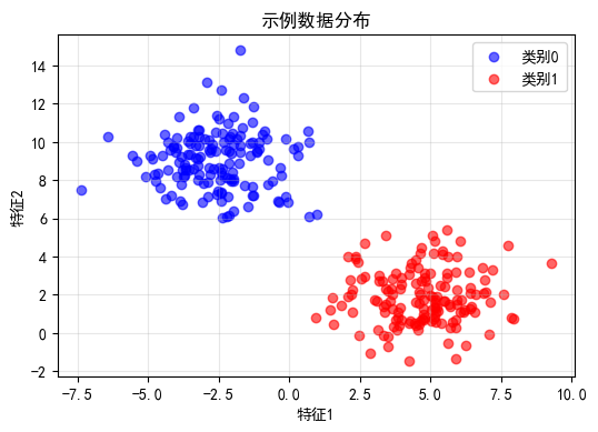

4.2 可视化决策树结构

# 绘制决策树
plt.figure(figsize=(8, 4))
plot_tree(tree_viz, filled=True, feature_names=['特征1', '特征2'], 
          class_names=['类别0', '类别1'], rounded=True, fontsize=10)
plt.title('决策树可视化', fontsize=16)
plt.show()

# 打印文本形式的决策树
print("决策树规则（文本形式）:")
print(export_text(tree_viz, feature_names=['特征1', '特征2']))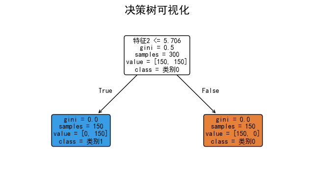

决策树规则（文本形式）:
|--- 特征2 <= 5.71
|   |--- class: 1
|--- 特征2 >  5.71
|   |--- class: 0

​

4.3 决策边界可视化

def plot_decision_boundary_tree(model, X, y, title="决策边界"):
    """可视化决策树的决策边界"""
    # 创建网格
    x_min, x_max = X[:, 0].min() - 1, X[:, 0].max() + 1
    y_min, y_max = X[:, 1].min() - 1, X[:, 1].max() + 1
    xx, yy = np.meshgrid(np.arange(x_min, x_max, 0.02),
                         np.arange(y_min, y_max, 0.02))
    
    # 预测网格点
    Z = model.predict(np.c_[xx.ravel(), yy.ravel()])
    Z = Z.reshape(xx.shape)
    
    # 绘图
    plt.figure(figsize=(10, 4))
    
    plt.subplot(1, 2, 1)
    plt.contourf(xx, yy, Z, alpha=0.3, cmap='RdYlBu')
    plt.scatter(X[y==0, 0], X[y==0, 1], c='blue', label='类别0', alpha=0.6, edgecolors='k')
    plt.scatter(X[y==1, 0], X[y==1, 1], c='red', label='类别1', alpha=0.6, edgecolors='k')
    plt.xlabel('特征1')
    plt.ylabel('特征2')
    plt.title(f'{title}\n(决策边界)')
    plt.legend()
    plt.grid(True, alpha=0.3)
    
    plt.subplot(1, 2, 2)
    # 绘制特征重要性
    importances = model.feature_importances_
    plt.bar(['特征1', '特征2'], importances)
    plt.xlabel('特征')
    plt.ylabel('重要性')
    plt.title('特征重要性')
    for i, imp in enumerate(importances):
        plt.text(i, imp + 0.01, f'{imp:.3f}', ha='center')
    
    plt.tight_layout()
    plt.show()

plot_decision_boundary_tree(tree_viz, X_blob, y_blob, "决策树决策边界")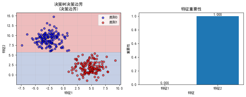

5. 过拟合实验：不同max_depth的影响

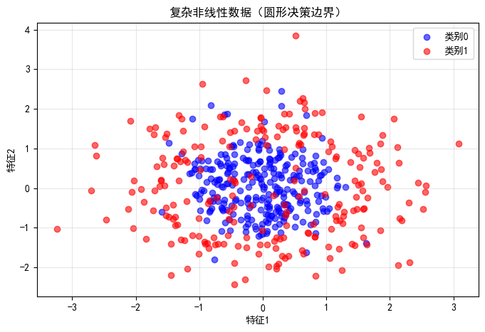
5.1 生成非线性数据

# 生成复杂的非线性数据
np.random.seed(42)
n_samples = 500
X_complex = np.random.randn(n_samples, 2)
y_complex = ((X_complex[:, 0]**2 + X_complex[:, 1]**2) > 1.5).astype(int)

# 添加一些噪声
noise_idx = np.random.choice(n_samples, int(n_samples * 0.1), replace=False)
y_complex[noise_idx] = 1 - y_complex[noise_idx]

# 可视化
plt.figure(figsize=(8, 5))
plt.scatter(X_complex[y_complex==0, 0], X_complex[y_complex==0, 1], 
            c='blue', label='类别0', alpha=0.6)
plt.scatter(X_complex[y_complex==1, 0], X_complex[y_complex==1, 1], 
            c='red', label='类别1', alpha=0.6)
plt.xlabel('特征1')
plt.ylabel('特征2')
plt.title('复杂非线性数据（圆形决策边界）')
plt.legend()
plt.grid(True, alpha=0.3)
plt.show()

# 划分数据
X_train_c, X_test_c, y_train_c, y_test_c = train_test_split(
    X_complex, y_complex, test_size=0.3, random_state=42
)

5.2 不同深度对比实验

def compare_depths(X_train, X_test, y_train, y_test, depths=[1, 3, 5, 10, 20]):
    """对比不同深度的决策树性能"""
    fig, axes = plt.subplots(2, 3, figsize=(15, 10))
    axes = axes.ravel()
    
    train_scores = []
    test_scores = []
    tree_models = []
    
    for idx, depth in enumerate(depths):
        # 训练决策树
        tree = DecisionTreeClassifier(max_depth=depth, random_state=42)
        tree.fit(X_train, y_train)
        tree_models.append(tree)
        
        # 计算准确率
        train_acc = accuracy_score(y_train, tree.predict(X_train))
        test_acc = accuracy_score(y_test, tree.predict(X_test))
        train_scores.append(train_acc)
        test_scores.append(test_acc)
        
        # 可视化决策边界
        x_min, x_max = X_train[:, 0].min() - 1, X_train[:, 0].max() + 1
        y_min, y_max = X_train[:, 1].min() - 1, X_train[:, 1].max() + 1
        xx, yy = np.meshgrid(np.arange(x_min, x_max, 0.05),
                             np.arange(y_min, y_max, 0.05))
        Z = tree.predict(np.c_[xx.ravel(), yy.ravel()])
        Z = Z.reshape(xx.shape)
        
        axes[idx].contourf(xx, yy, Z, alpha=0.3, cmap='RdYlBu')
        axes[idx].scatter(X_train[y_train==0, 0], X_train[y_train==0, 1], 
                         c='blue', alpha=0.4, s=20)
        axes[idx].scatter(X_train[y_train==1, 0], X_train[y_train==1, 1], 
                         c='red', alpha=0.4, s=20)
        axes[idx].set_title(f'max_depth={depth}\n训练集: {train_acc:.3f} | 测试集: {test_acc:.3f}')
        axes[idx].set_xlabel('特征1')
        axes[idx].set_ylabel('特征2')
        
        # 计算树的信息
        n_nodes = tree.tree_.node_count
        n_leaves = tree.get_n_leaves()
        axes[idx].text(0.05, 0.95, f'节点数: {n_nodes}\n叶节点数: {n_leaves}',
                      transform=axes[idx].transAxes, fontsize=9,
                      verticalalignment='top', bbox=dict(boxstyle='round', facecolor='wheat', alpha=0.5))
    
    # 隐藏多余的子图
    for idx in range(len(depths), len(axes)):
        axes[idx].set_visible(False)
    
    plt.tight_layout()
    plt.show()
    
    # 绘制性能曲线
    plt.figure(figsize=(8, 5))
    plt.plot(depths, train_scores, 'b-o', label='训练集准确率', linewidth=2, markersize=8)
    plt.plot(depths, test_scores, 'r-s', label='测试集准确率', linewidth=2, markersize=8)
    plt.xlabel('树的最大深度 (max_depth)')
    plt.ylabel('准确率')
    plt.title('决策树深度对性能的影响（过拟合可视化）')
    plt.legend()
    plt.grid(True, alpha=0.3)
    
    # 标注过拟合区域
    best_depth = depths[np.argmax(test_scores)]
    plt.axvline(x=best_depth, color='g', linestyle='--', label=f'最佳深度={best_depth}')
    
    # 添加注解
    plt.annotate('欠拟合区域', xy=(1, 0.7), xytext=(2, 0.6),
                arrowprops=dict(arrowstyle='->', color='orange'))
    plt.annotate('过拟合区域', xy=(20, 0.7), xytext=(15, 0.55),
                arrowprops=dict(arrowstyle='->', color='orange'))
    
    plt.legend()
    plt.show()
    
    print(f"最佳深度: {best_depth}")
    print(f"最佳测试准确率: {max(test_scores):.4f}")
    
    return tree_models, train_scores, test_scores

# 执行对比实验
trees, train_scores, test_scores = compare_depths(
    X_train_c, X_test_c, y_train_c, y_test_c,
    depths=[1, 2, 3, 5, 10, 20]
)

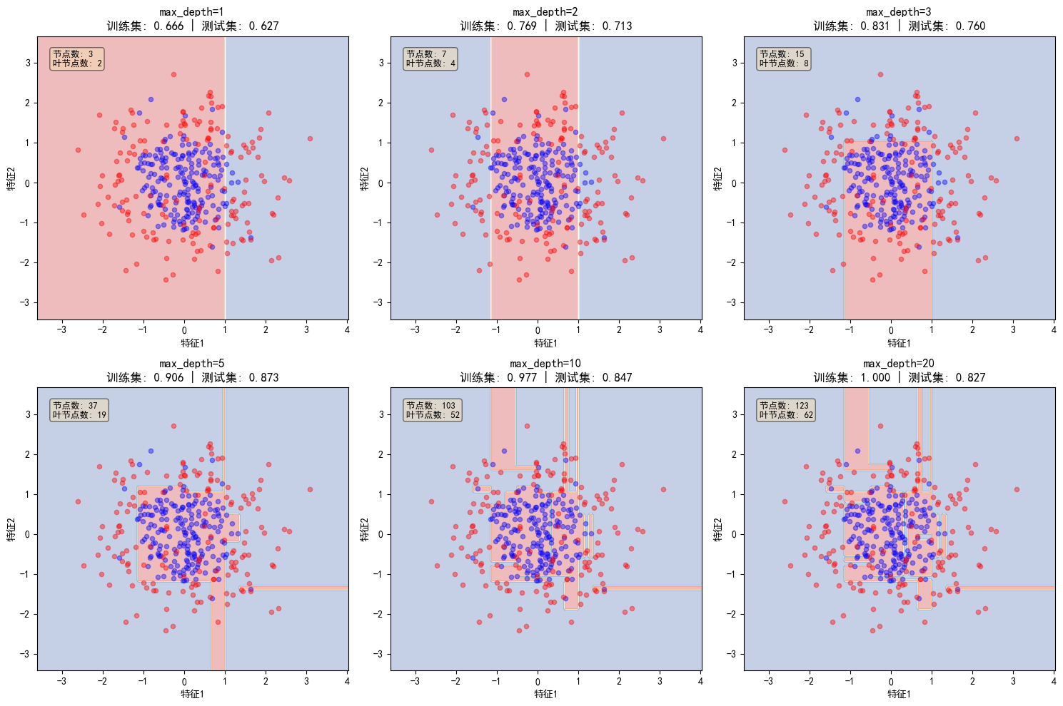
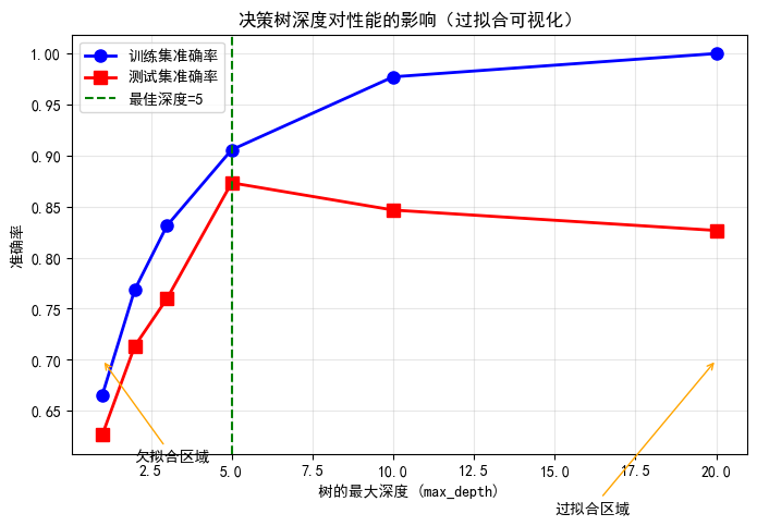
最佳深度: 5
最佳测试准确率: 0.8733

5.3 过拟合详细分析

def analyze_overfitting(X_train, X_test, y_train, y_test, max_depth=20):
    """详细分析过拟合现象"""
    
    # 训练不同深度的树
    depths = range(1, max_depth + 1)
    train_accuracies = []
    test_accuracies = []
    tree_sizes = []
    
    for depth in depths:
        tree = DecisionTreeClassifier(max_depth=depth, random_state=42)
        tree.fit(X_train, y_train)
        train_accuracies.append(accuracy_score(y_train, tree.predict(X_train)))
        test_accuracies.append(accuracy_score(y_test, tree.predict(X_test)))
        tree_sizes.append(tree.tree_.node_count)
    
    # 创建可视化
    fig, axes = plt.subplots(1, 3, figsize=(15, 4))
    
    # 准确率曲线
    axes[0].plot(depths, train_accuracies, 'b-', label='训练集', linewidth=2)
    axes[0].plot(depths, test_accuracies, 'r-', label='测试集', linewidth=2)
    axes[0].fill_between(depths, train_accuracies, test_accuracies, 
                         where=(np.array(train_accuracies) > np.array(test_accuracies)),
                         alpha=0.3, color='red', label='过拟合差距')
    axes[0].set_xlabel('树深度')
    axes[0].set_ylabel('准确率')
    axes[0].set_title('训练集 vs 测试集准确率')
    axes[0].legend()
    axes[0].grid(True, alpha=0.3)
    
    # 过拟合差距
    gap = np.array(train_accuracies) - np.array(test_accuracies)
    axes[1].plot(depths, gap, 'g-o', linewidth=2)
    axes[1].axhline(y=0, color='k', linestyle='--')
    axes[1].fill_between(depths, 0, gap, where=(gap > 0), alpha=0.3, color='red')
    axes[1].set_xlabel('树深度')
    axes[1].set_ylabel('训练-测试准确率差')
    axes[1].set_title('过拟合程度（差距越大，过拟合越严重）')
    axes[1].grid(True, alpha=0.3)
    
    # 树的大小
    axes[2].plot(depths, tree_sizes, 'm-o', linewidth=2)
    axes[2].set_xlabel('树深度')
    axes[2].set_ylabel('节点数')
    axes[2].set_title('决策树复杂度随深度增长')
    axes[2].grid(True, alpha=0.3)
    
    plt.tight_layout()
    plt.show()
    
    # 打印关键观察
    print("\n" + "="*60)
    print("过拟合分析结论")
    print("="*60)
    best_depth = depths[np.argmax(test_accuracies)]
    print(f"1. 最佳深度: {best_depth}")
    print(f"2. 最佳测试准确率: {max(test_accuracies):.4f}")
    print(f"3. 深度{max_depth}时的过拟合差距: {gap[-1]:.4f}")
    print(f"4. 深度从{best_depth}增加到{max_depth}:")
    print(f"   - 训练准确率提升: {train_accuracies[-1] - train_accuracies[best_depth-1]:.2%}")
    print(f"   - 测试准确率下降: {test_accuracies[best_depth-1] - test_accuracies[-1]:.2%}")
    print(f"   - 节点数增加: {tree_sizes[-1] - tree_sizes[best_depth-1]}")

analyze_overfitting(X_train_c, X_test_c, y_train_c, y_test_c, max_depth=20)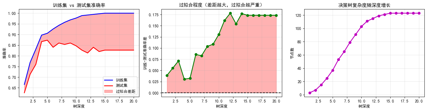

​

============================================================

过拟合分析结论

============================================================

1. 最佳深度: 5

2. 最佳测试准确率: 0.8733

3. 深度20时的过拟合差距: 0.1733

4. 深度从5增加到20:

• 训练准确率提升: 9.43%

• 测试准确率下降: 4.67%

• 节点数增加: 86

6. 金融应用：预测股票涨跌

6.1 加载股票K线数据

from pathlib import Path

def read_stock_data(ts_code):
    """生成模拟股票数据，包含多种形态"""

    data_path = Path(r"E:\AppData\quant_trade\klines\kline2014-2024")
    kline_file = data_path / f"{ts_code}.csv"
    
    df = pd.read_csv(kline_file, usecols=["trade_date", "close", "vol"],
                     parse_dates=["trade_date"]).sort_values(by=["trade_date"]).reset_index(drop=True)
    
    # 计算收益率
    df['return'] = df['close'].pct_change()

    # RSI
    delta = df['return'].fillna(0)
    gain = delta.where(delta > 0, 0).rolling(14).mean()
    loss = -delta.where(delta < 0, 0).rolling(14).mean()
    rs = gain / (loss + 1e-10)
    df['rsi'] = 100 - (100 / (1 + rs))

    # MACD
    ema12 = df['close'].ewm(span=12, adjust=False).mean()
    ema26 = df['close'].ewm(span=26, adjust=False).mean()
    df['macd'] = ema12 - ema26
    df['macd_signal'] = df['macd'].ewm(span=9, adjust=False).mean()
    df['macd_hist'] = df['macd'] - df['macd_signal']
    
    # 移动平均线
    df['ma5'] = df['close'].rolling(5).mean()
    df['ma20'] = df['close'].rolling(20).mean()
    df['ma_ratio'] = df['ma5'] / df['ma20'] - 1
    
    # 波动率
    df['volatility'] = df['return'].rolling(20).std()
    
    # 成交量指标
    df['volume_ma'] = df['vol'].rolling(10).mean()
    df['volume_ratio'] = df['vol'] / df['volume_ma']
    
    # 目标变量：3日是否上涨
    df['target'] = (df['close'].shift(-3) > df['close']).astype(int)
    
    return df.dropna()

# 生成数据
df_finance = read_stock_data("600519.SH")
print(f"数据形状: {df_finance.shape}")
df_finance.head()

# 查看数据分布
print("\n目标变量分布:")
print(df_finance['target'].value_counts(normalize=True))

数据形状: (2452, 15)

目标变量分布:
target
1    0.544454
0    0.455546
Name: proportion, dtype: float64

6.2 特征选择与数据划分

# 选择特征
feature_cols = ['rsi', 'macd', 'macd_hist', 'ma_ratio', 'volatility', 'volume_ratio']
X_fin = df_finance[feature_cols]
y_fin = df_finance['target']

# 按时间划分（避免前视偏差）
split_idx = int(len(df_finance) * 0.7)
X_train_f = X_fin[:split_idx]
X_test_f = X_fin[split_idx:]
y_train_f = y_fin[:split_idx]
y_test_f = y_fin[split_idx:]

print(f"训练集大小: {len(X_train_f)}")
print(f"测试集大小: {len(X_test_f)}")
print(f"训练集正样本比例: {y_train_f.mean():.2%}")

训练集大小: 1716
测试集大小: 736
训练集正样本比例: 57.28%

6.3 训练不同深度的决策树

# 训练不同深度的决策树
depths_fin = [2, 3, 5, 7, 10, 15]
train_scores_fin = []
test_scores_fin = []

for depth in depths_fin:
    tree = DecisionTreeClassifier(max_depth=depth, random_state=42)
    tree.fit(X_train_f, y_train_f)
    
    train_acc = accuracy_score(y_train_f, tree.predict(X_train_f))
    test_acc = accuracy_score(y_test_f, tree.predict(X_test_f))
    train_scores_fin.append(train_acc)
    test_scores_fin.append(test_acc)
    
    print(f"max_depth={depth:2d} | 训练集: {train_acc:.4f} | 测试集: {test_acc:.4f}")

# 可视化
plt.figure(figsize=(10, 4))

plt.subplot(1, 2, 1)
plt.plot(depths_fin, train_scores_fin, 'b-o', label='训练集', linewidth=2)
plt.plot(depths_fin, test_scores_fin, 'r-s', label='测试集', linewidth=2)
plt.xlabel('树深度')
plt.ylabel('准确率')
plt.title('金融数据预测 - 不同深度性能对比')
plt.legend()
plt.grid(True, alpha=0.3)

# 最佳深度
best_depth_fin = depths_fin[np.argmax(test_scores_fin)]
plt.axvline(x=best_depth_fin, color='g', linestyle='--', label=f'最佳深度={best_depth_fin}')
plt.legend()

# 过拟合差距
plt.subplot(1, 2, 2)
gap = np.array(train_scores_fin) - np.array(test_scores_fin)
plt.bar([str(d) for d in depths_fin], gap, color=['green' if g < 0.05 else 'orange' if g < 0.1 else 'red' for g in gap])
plt.xlabel('树深度')
plt.ylabel('训练-测试准确率差')
plt.title('过拟合程度分析')
plt.axhline(y=0.05, color='green', linestyle='--', label='可接受差距')
plt.axhline(y=0.1, color='red', linestyle='--', label='严重过拟合')
plt.legend()

plt.tight_layout()
plt.show()

max_depth= 2 | 训练集: 0.5903 | 测试集: 0.4905
max_depth= 3 | 训练集: 0.5903 | 测试集: 0.4905
max_depth= 5 | 训练集: 0.6090 | 测试集: 0.5408
max_depth= 7 | 训练集: 0.6457 | 测试集: 0.5095
max_depth=10 | 训练集: 0.7273 | 测试集: 0.4796
max_depth=15 | 训练集: 0.8829 | 测试集: 0.5000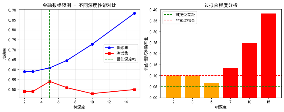

6.4 特征重要性分析

# 使用最佳深度的树
best_tree = DecisionTreeClassifier(max_depth=best_depth_fin, random_state=42)
best_tree.fit(X_train_f, y_train_f)

# 特征重要性
importances = best_tree.feature_importances_
feature_importance_df = pd.DataFrame({
    'Feature': feature_cols,
    'Importance': importances
}).sort_values('Importance', ascending=False)

plt.figure(figsize=(10, 6))
plt.barh(feature_importance_df['Feature'], feature_importance_df['Importance'])
plt.xlabel('重要性')
plt.ylabel('特征')
plt.title(f'决策树特征重要性 (max_depth={best_depth_fin})')
for i, (_, row) in enumerate(feature_importance_df.iterrows()):
    plt.text(row['Importance'] + 0.01, i, f"{row['Importance']:.3f}", va='center')
plt.grid(True, alpha=0.3)
plt.show()

print("特征重要性排序:")
print(feature_importance_df.to_string(index=False))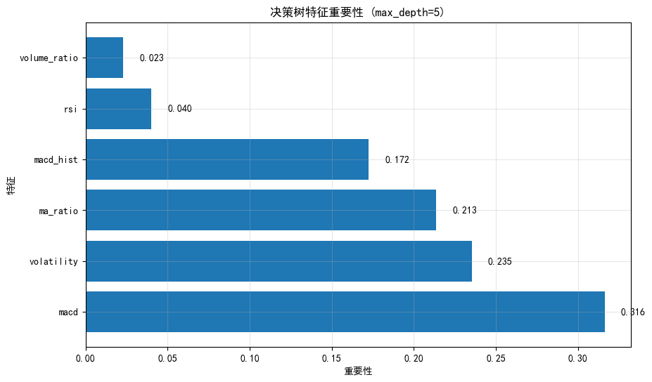

特征重要性排序:
     Feature  Importance
        macd    0.316185
  volatility    0.235141
    ma_ratio    0.213499
   macd_hist    0.172273
         rsi    0.039951
volume_ratio    0.022951

6.5 决策树规则提取

# 提取决策树规则
tree_rules = export_text(best_tree, feature_names=feature_cols)
print("决策树规则（可解释的交易信号）:")
print("="*60)
print(tree_rules)

# 可视化树结构（简化版）
plt.figure(figsize=(10, 6))
plot_tree(best_tree, feature_names=feature_cols, class_names=['下跌', '上涨'],
          filled=True, rounded=True, fontsize=8, max_depth=3)  # 只显示前3层避免拥挤
plt.title(f'金融预测决策树可视化 (max_depth={best_depth_fin})', fontsize=16)
plt.tight_layout()
plt.show()

决策树规则（可解释的交易信号）:
============================================================
|--- volatility <= 0.03
|   |--- ma_ratio <= -0.04
|   |   |--- macd_hist <= -4.66
|   |   |   |--- class: 1
|   |   |--- macd_hist >  -4.66
|   |   |   |--- volatility <= 0.02
|   |   |   |   |--- class: 0
|   |   |   |--- volatility >  0.02
|   |   |   |   |--- macd <= -17.49
|   |   |   |   |   |--- class: 0
|   |   |   |   |--- macd >  -17.49
|   |   |   |   |   |--- class: 1
|   |--- ma_ratio >  -0.04
|   |   |--- macd <= 13.59
|   |   |   |--- macd_hist <= 0.79
|   |   |   |   |--- volatility <= 0.02
|   |   |   |   |   |--- class: 1
|   |   |   |   |--- volatility >  0.02
|   |   |   |   |   |--- class: 0
|   |   |   |--- macd_hist >  0.79
|   |   |   |   |--- ma_ratio <= -0.01
|   |   |   |   |   |--- class: 1
|   |   |   |   |--- ma_ratio >  -0.01
|   |   |   |   |   |--- class: 0
|   |   |--- macd >  13.59
|   |   |   |--- macd <= 86.25
|   |   |   |   |--- macd <= 39.93
|   |   |   |   |   |--- class: 1
|   |   |   |   |--- macd >  39.93
|   |   |   |   |   |--- class: 1
|   |   |   |--- macd >  86.25
|   |   |   |   |--- macd_hist <= 24.36
|   |   |   |   |   |--- class: 0
|   |   |   |   |--- macd_hist >  24.36
|   |   |   |   |   |--- class: 0
|--- volatility >  0.03
|   |--- macd_hist <= -13.17
|   |   |--- class: 1
|   |--- macd_hist >  -13.17
|   |   |--- macd <= 32.60
|   |   |   |--- rsi <= 34.04
|   |   |   |   |--- volume_ratio <= 0.48
|   |   |   |   |   |--- class: 0
|   |   |   |   |--- volume_ratio >  0.48
|   |   |   |   |   |--- class: 1
|   |   |   |--- rsi >  34.04
|   |   |   |   |--- macd <= 30.78
|   |   |   |   |   |--- class: 0
|   |   |   |   |--- macd >  30.78
|   |   |   |   |   |--- class: 1
|   |   |--- macd >  32.60
|   |   |   |--- class: 0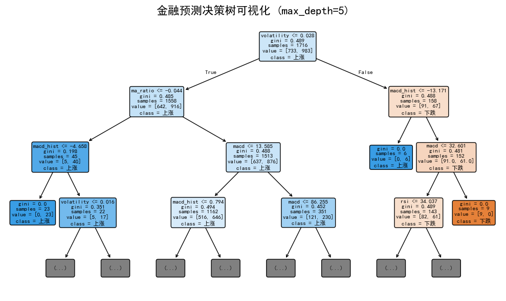

7. 剪枝参数优化

7.1 预剪枝参数实验

def experiment_pre_pruning(X_train, X_test, y_train, y_test):
    """实验不同的预剪枝参数"""
    
    # 参数组合
    param_tests = [
        {'name': '无限制', 'params': {'max_depth': None, 'min_samples_split': 2, 'min_samples_leaf': 1}},
        {'name': 'max_depth=5', 'params': {'max_depth': 5, 'min_samples_split': 2, 'min_samples_leaf': 1}},
        {'name': 'max_depth=10', 'params': {'max_depth': 10, 'min_samples_split': 2, 'min_samples_leaf': 1}},
        {'name': 'min_samples_split=20', 'params': {'max_depth': None, 'min_samples_split': 20, 'min_samples_leaf': 1}},
        {'name': 'min_samples_leaf=10', 'params': {'max_depth': None, 'min_samples_split': 2, 'min_samples_leaf': 10}},
        {'name': '严格限制', 'params': {'max_depth': 5, 'min_samples_split': 20, 'min_samples_leaf': 10}}
    ]
    
    results = []
    
    for test in param_tests:
        tree = DecisionTreeClassifier(**test['params'], random_state=42)
        tree.fit(X_train, y_train)
        
        train_acc = accuracy_score(y_train, tree.predict(X_train))
        test_acc = accuracy_score(y_test, tree.predict(X_test))
        n_nodes = tree.tree_.node_count
        
        results.append({
            '配置': test['name'],
            '训练集准确率': train_acc,
            '测试集准确率': test_acc,
            '节点数': n_nodes,
            '过拟合差距': train_acc - test_acc
        })
    
    results_df = pd.DataFrame(results)
    print(results_df.to_string(index=False))
    
    # 可视化
    fig, axes = plt.subplots(1, 2, figsize=(10, 4))
    
    x = range(len(results))
    axes[0].bar(x, results_df['测试集准确率'], color='green', alpha=0.7, label='测试集')
    axes[0].bar(x, results_df['训练集准确率'], color='blue', alpha=0.5, label='训练集', width=0.5)
    axes[0].set_xticks(x)
    axes[0].set_xticklabels(results_df['配置'], rotation=45, ha='right')
    axes[0].set_ylabel('准确率')
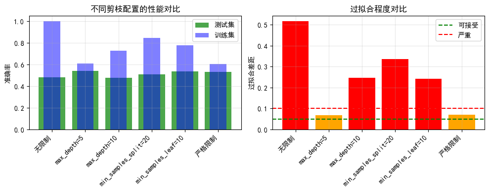
    axes[0].set_title('不同剪枝配置的性能对比')
    axes[0].legend()
    axes[0].grid(True, alpha=0.3)
    
    axes[1].bar(x, results_df['过拟合差距'], color=['green' if g < 0.05 else 'orange' if g < 0.1 else 'red' for g in results_df['过拟合差距']])
    axes[1].set_xticks(x)
    axes[1].set_xticklabels(results_df['配置'], rotation=45, ha='right')
    axes[1].set_ylabel('过拟合差距')
    axes[1].set_title('过拟合程度对比')
    axes[1].axhline(y=0.05, color='green', linestyle='--', label='可接受')
    axes[1].axhline(y=0.1, color='red', linestyle='--', label='严重')
    axes[1].legend()
    axes[1].grid(True, alpha=0.3)
    
    plt.tight_layout()
    plt.show()
    
    return results_df

# 执行实验
pruning_results = experiment_pre_pruning(X_train_f, X_test_f, y_train_f, y_test_f)

配置	训练集准确率	测试集准确率	节点数	过拟合差距
无限制	1.000000	0.483696	803	0.516304
max_depth=5	0.608974	0.540761	35	0.068213
max_depth=10	0.727273	0.479620	207	0.247653
min_samples_split=20	0.847319	0.510870	357	0.336450
min_samples_leaf=10	0.780886	0.539402	255	0.241484
严格限制	0.605478	0.533967	29	0.071510

7.2 成本复杂度剪枝（CCP）

def ccp_pruning_demo(X_train, X_test, y_train, y_test):
    """演示成本复杂度剪枝"""
    
    # 先构建一个不剪枝的完整树
    tree_full = DecisionTreeClassifier(random_state=42)
    tree_full.fit(X_train, y_train)
    
    # 获取剪枝路径
    path = tree_full.cost_complexity_pruning_path(X_train, y_train)
    ccp_alphas = path.ccp_alphas
    impurities = path.impurities
    
    # 对不同alpha训练树
    trees_ccp = []
    train_scores_ccp = []
    test_scores_ccp = []
    
    for alpha in ccp_alphas[:-1]:  # 排除最后一个（会变成单节点）
        tree = DecisionTreeClassifier(ccp_alpha=alpha, random_state=42)
        tree.fit(X_train, y_train)
        trees_ccp.append(tree)
        train_scores_ccp.append(accuracy_score(y_train, tree.predict(X_train)))
        test_scores_ccp.append(accuracy_score(y_test, tree.predict(X_test)))
    
    # 可视化
    fig, axes = plt.subplots(1, 2, figsize=(10, 4))
    
    # 剪枝路径
    axes[0].plot(ccp_alphas[:-1], impurities[:-1], 'b-o', linewidth=2)
    axes[0].set_xlabel('ccp_alpha')
    axes[0].set_ylabel('总不纯度')
    axes[0].set_title('成本复杂度剪枝路径')
    axes[0].grid(True, alpha=0.3)
    
    # 性能随alpha变化
    axes[1].plot(ccp_alphas[:-1], train_scores_ccp, 'b-o', label='训练集', linewidth=2)
    axes[1].plot(ccp_alphas[:-1], test_scores_ccp, 'r-s', label='测试集', linewidth=2)
    axes[1].set_xlabel('ccp_alpha')
    axes[1].set_ylabel('准确率')
    axes[1].set_title('CCP剪枝效果')
    axes[1].legend()
    axes[1].grid(True, alpha=0.3)
    
    # 标记最佳alpha
    best_idx = np.argmax(test_scores_ccp)
    best_alpha = ccp_alphas[best_idx]
    axes[1].axvline(x=best_alpha, color='g', linestyle='--', label=f'最佳alpha={best_alpha:.4f}')
    axes[1].legend()
    
    plt.tight_layout()
    plt.show()
    
    print(f"最佳ccp_alpha: {best_alpha:.6f}")
    print(f"最佳测试准确率: {max(test_scores_ccp):.4f}")
    print(f"原始树测试准确率: {test_scores_ccp[0]:.4f}")
    print(f"剪枝后提升: {(max(test_scores_ccp) - test_scores_ccp[0])*100:.2f}%")
    
    return best_alpha

best_alpha = ccp_pruning_demo(X_train_f, X_test_f, y_train_f, y_test_f)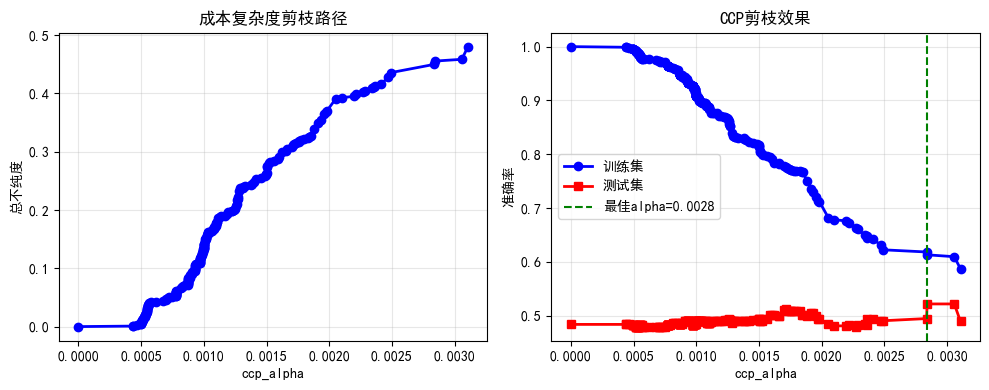

最佳ccp_alpha: 0.002840
最佳测试准确率: 0.5217
原始树测试准确率: 0.4837
剪枝后提升: 3.80%

8. 交叉验证选择最佳参数

8.1 网格搜索

from sklearn.model_selection import GridSearchCV

# 参数网格
param_grid = {
    'max_depth': [3, 5, 7, 10, 15],
    'min_samples_split': [2, 5, 10, 20],
    'min_samples_leaf': [1, 2, 5, 10],
    'criterion': ['gini', 'entropy']
}

# 网格搜索
tree_gs = DecisionTreeClassifier(random_state=42)
grid_search = GridSearchCV(tree_gs, param_grid, cv=5, scoring='accuracy', n_jobs=-1)
grid_search.fit(X_train_f, y_train_f)

print("最佳参数组合:")
print(grid_search.best_params_)
print(f"\n最佳交叉验证准确率: {grid_search.best_score_:.4f}")
print(f"测试集准确率: {accuracy_score(y_test_f, grid_search.predict(X_test_f)):.4f}")

# 使用最佳模型
best_tree_cv = grid_search.best_estimator_

最佳参数组合:
{'criterion': 'entropy', 'max_depth': 3, 'min_samples_leaf': 1, 'min_samples_split': 2}

最佳交叉验证准确率: 0.5641
测试集准确率: 0.4905

8.2 最佳模型评估

y_pred_best = best_tree_cv.predict(X_test_f)
y_pred_proba = best_tree_cv.predict_proba(X_test_f)[:, 1]

# 混淆矩阵
cm = confusion_matrix(y_test_f, y_pred_best)

plt.figure(figsize=(8, 3))

plt.subplot(1, 2, 1)
sns.heatmap(cm, annot=True, fmt='d', cmap='Blues',
            xticklabels=['预测下跌', '预测上涨'],
            yticklabels=['实际下跌', '实际上涨'])
plt.title('混淆矩阵 - 最佳决策树')

plt.subplot(1, 2, 2)
# 特征重要性
importances_best = best_tree_cv.feature_importances_
plt.barh(feature_cols, importances_best)
plt.xlabel('重要性')
plt.title('特征重要性')

plt.tight_layout()
plt.show()

print("\n分类报告:")
print(classification_report(y_test_f, y_pred_best, target_names=['下跌', '上涨']))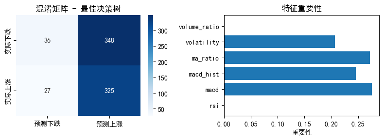

​

分类报告:

                 precision    recall  f1-score   support

          下跌       0.57      0.09      0.16       384
          上涨       0.48      0.92      0.63       352

      accuracy                           0.49       736
     macro avg       0.53      0.51      0.40       736
  weighted avg       0.53      0.49      0.39       736

​

9. 决策树 vs 随机森林（预告）

9.1 简单对比

from sklearn.ensemble import RandomForestClassifier

# 单棵决策树
single_tree = DecisionTreeClassifier(max_depth=5, random_state=42)
single_tree.fit(X_train_f, y_train_f)

# 随机森林
rf = RandomForestClassifier(n_estimators=100, max_depth=5, random_state=42)
rf.fit(X_train_f, y_train_f)

# 对比
print("="*60)
print("决策树 vs 随机森林对比")
print("="*60)
print(f"决策树 - 训练集: {accuracy_score(y_train_f, single_tree.predict(X_train_f)):.4f}")
print(f"决策树 - 测试集: {accuracy_score(y_test_f, single_tree.predict(X_test_f)):.4f}")
print(f"随机森林 - 训练集: {accuracy_score(y_train_f, rf.predict(X_train_f)):.4f}")
print(f"随机森林 - 测试集: {accuracy_score(y_test_f, rf.predict(X_test_f)):.4f}")

# 可视化对比
plt.figure(figsize=(6, 3))
models = ['决策树', '随机森林']
train_scores_compare = [
    accuracy_score(y_train_f, single_tree.predict(X_train_f)),
    accuracy_score(y_train_f, rf.predict(X_train_f))
]
test_scores_compare = [
    accuracy_score(y_test_f, single_tree.predict(X_test_f)),
    accuracy_score(y_test_f, rf.predict(X_test_f))
]

x = np.arange(len(models))
width = 0.35
plt.bar(x - width/2, train_scores_compare, width, label='训练集', alpha=0.8)
plt.bar(x + width/2, test_scores_compare, width, label='测试集', alpha=0.8)
plt.xlabel('模型')
plt.ylabel('准确率')
plt.title('决策树 vs 随机森林')
plt.xticks(x, models)
plt.legend()
plt.grid(True, alpha=0.3)
plt.show()

============================================================
决策树 vs 随机森林对比
============================================================
决策树 - 训练集: 0.6090
决策树 - 测试集: 0.5408
随机森林 - 训练集: 0.6381
随机森林 - 测试集: 0.4823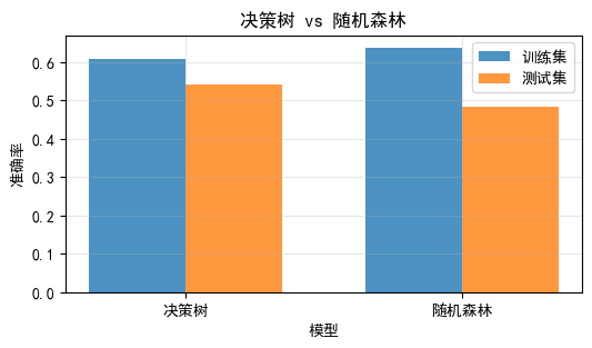

10. 今日总结与练习

核心要点回顾

决策树基础：

• 树形结构，可解释性强
• ID3用信息增益，CART用基尼系数
• 可以处理分类和回归任务

分裂准则：

• 信息增益：基于熵，计算较慢
• 基尼系数：计算快，效果相近
• 均方误差：回归树使用

过拟合控制：

• 预剪枝：限制深度、最小样本数
• 后剪枝：成本复杂度剪枝
• 使用交叉验证选择参数

量化应用：

• 可解释的交易规则
• 特征重要性帮助因子筛选
• 但需注意过拟合

今日练习

# 练习1：尝试不同的分裂准则（gini vs entropy），比较效果
# 练习2：使用export_text导出更详细的规则，转化为交易策略
# 练习3：实现回归树预测收益率
# 练习4：使用真实股票数据（yfinance）测试决策树策略

思考题

1. 决策树的可解释性在量化交易中有什么价值？
2. 如何避免决策树在金融数据中过拟合？
3. 从决策树中提取的规则可以直接用于交易吗？需要注意什么？

量化思考

今天的决策树如何应用到量化交易？

• 从树中提取if-then规则作为交易信号
• 分析特征重要性，优化因子组合
• 但要注意过拟合，使用适当的剪枝
• 可以与随机森林等集成方法对比