1 背景
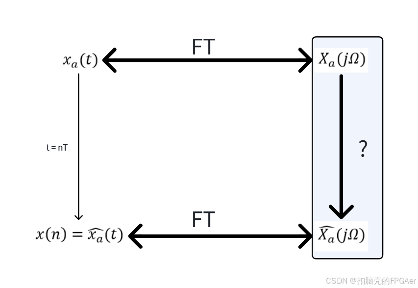
信号被采样后再频域会发生什么变化?
2 理想时域采样
2.1 采样
利用周期性理想冲击函数序列 ,从连续信号
 中抽取一系列的离散值,得到
2.2 采样器
类似于一个电子开关,开关每间隔T秒(采样间隔)闭合一次,使得时间离散
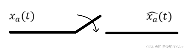
使用周期性理想冲击函数序列,以采样周期T等间隔采样,可以得到时域离散的信号
Matlab
clear; clc;
f0 = 5; fs = 200; Ts = 1/fs;
t_continuous = linspace(0, 1, 1000);
t_discrete = 0:Ts:1;
x_continuous = sin(2*pi*f0*t_continuous);
x_discrete = sin(2*pi*f0*t_discrete);
figure;
plot(t_continuous, x_continuous, 'b-', 'LineWidth', 1.5);
hold on;
stem(t_discrete, x_discrete, 'r', 'LineWidth', 2, ...
'MarkerSize', 8, 'MarkerFaceColor', 'r');
hold off;
grid on;
xlabel('时间 (s)');
ylabel('幅度');
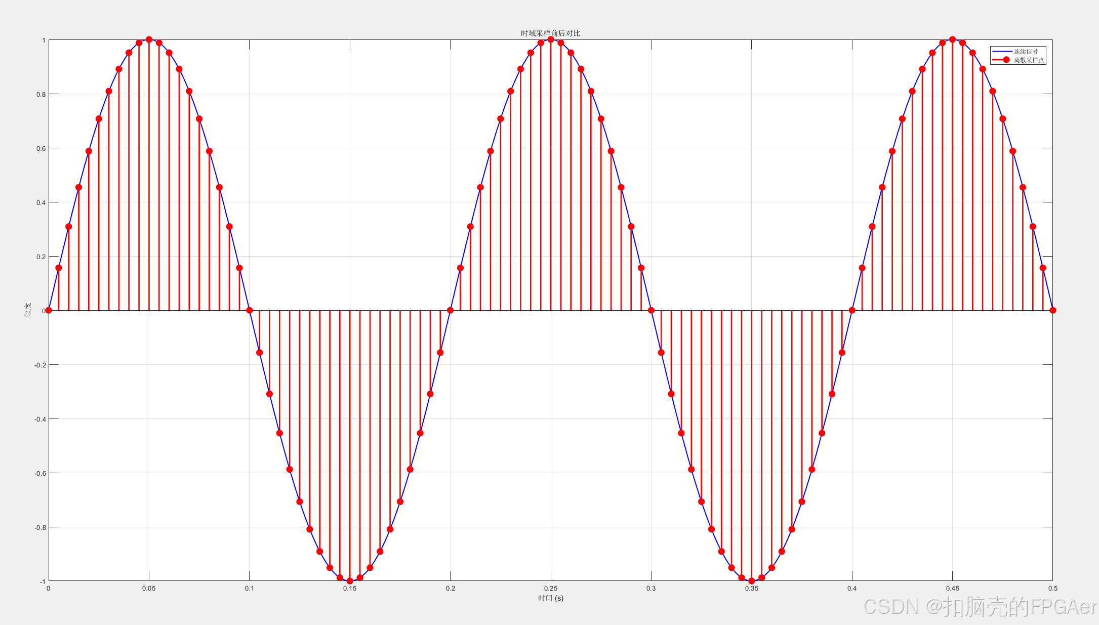
title('时域采样前后对比');
legend('连续信号', '离散采样点');
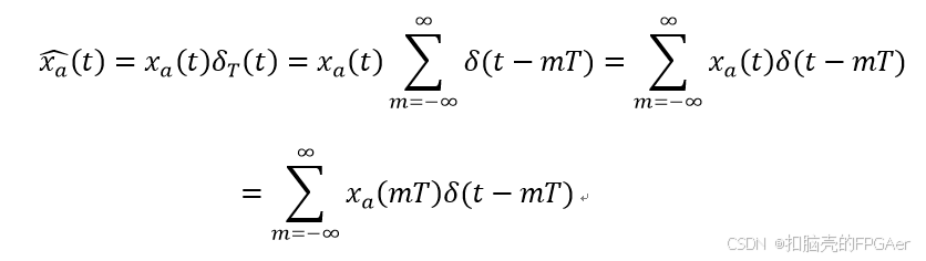
xlim([0, 0.5]);就理想采样而言,周期性冲激函数序列 的各冲激函数准确地出现在采样瞬间上,采样后的信号完全于输入信号在采样瞬间的幅度相同。
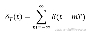
冲激函数序列:
理想采样输出:
Matlab
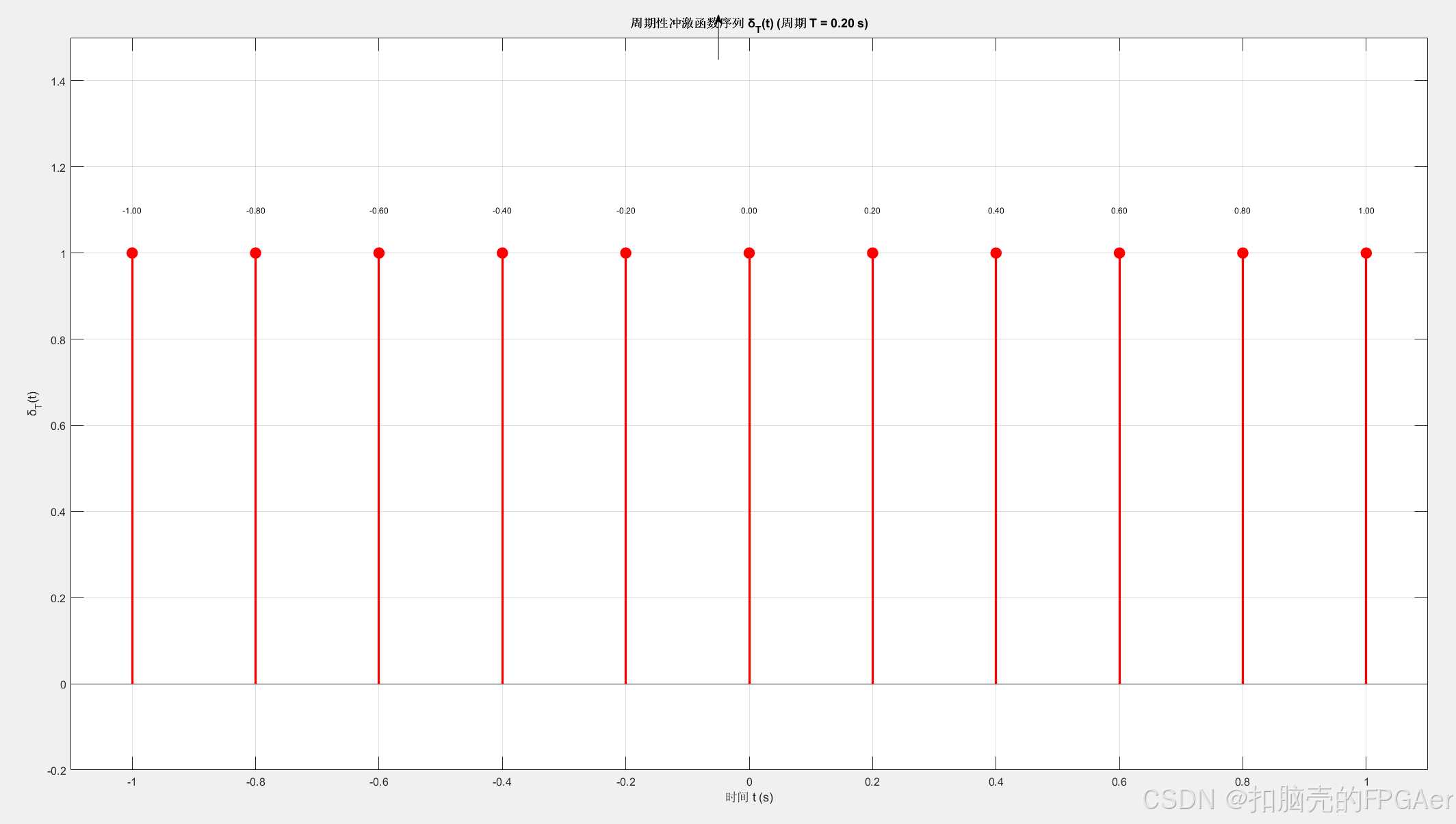
%% 绘制周期为T的周期性冲激函数序列 δ_T(t)
clear all; close all; clc;

%% 参数设置
T = 0.2;            % 周期 (s)
t_start = -1;       % 开始时间
t_end = 1;          % 结束时间
t_discrete = t_start:T:t_end;  % 冲激出现的时间点

% 冲激强度(理论上无穷大,图示中用1表示)
impulse_amplitude = 1;

%% 创建图形窗口
figure('Position', [100, 100, 1000, 600]);

% 绘制周期性冲激序列
stem(t_discrete, impulse_amplitude * ones(size(t_discrete)), 'r', ...
     'LineWidth', 2.5, 'MarkerSize', 10, 'MarkerFaceColor', 'r');
grid on;
xlabel('时间 t (s)', 'FontSize', 14);
ylabel('δ_T(t)', 'FontSize', 14);
title(sprintf('周期性冲激函数序列 δ_T(t) (周期 T = %.2f s)', T), ...
      'FontSize', 16, 'FontWeight', 'bold');
xlim([t_start-0.1, t_end+0.1]);
ylim([-0.2, 1.5]);
set(gca, 'FontSize', 12);

% 添加标注
for i = 1:length(t_discrete)
    text(t_discrete(i), 1.1, sprintf('%.2f', t_discrete(i)), ...
         'HorizontalAlignment', 'center', 'FontSize', 9);
end

% 添加箭头表示冲激
annotation('arrow', [0.5, 0.5], [0.9, 0.95]);
3 理想采样后信号频域变化
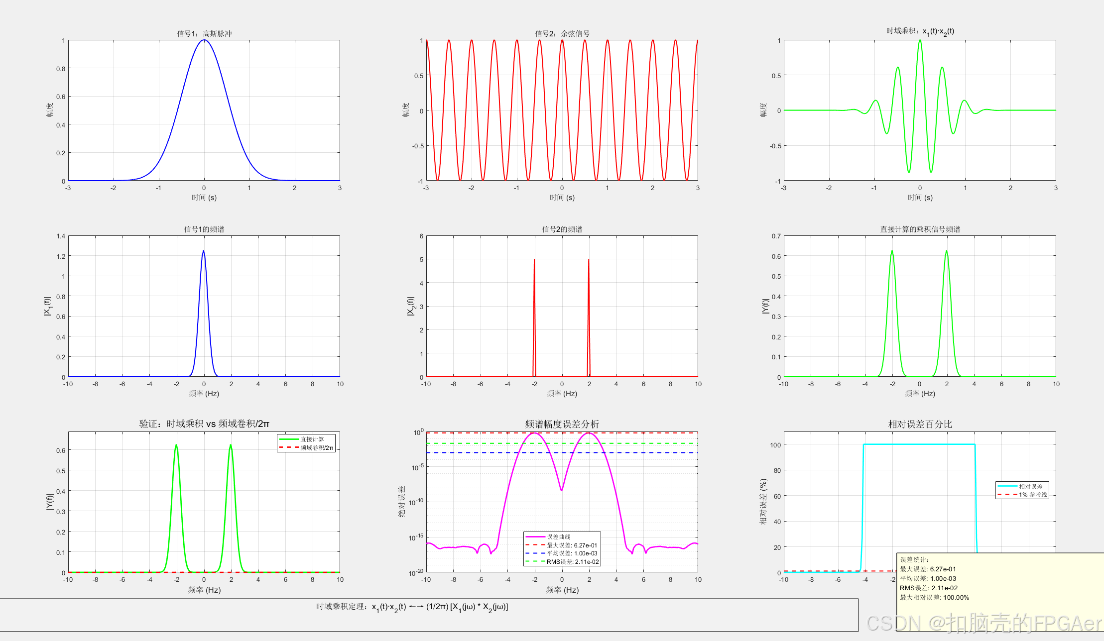
3.1 变化过程思考
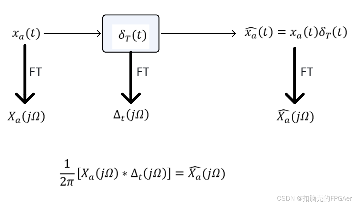
时序的乘积 <------> 1/2pi 乘以频域的卷积,注意这里的频域为什么要乘以1/2pi?
Matlab
clear all; close all; clc;

%% 参数设置
fs = 1000;          % 采样频率
t = -5:1/fs:5;      % 时间轴
N = length(t);
df = fs/N;
f = (-N/2:N/2-1)*df;

%% 定义两个信号
% 信号1:高斯脉冲
sigma1 = 0.5;
x1 = exp(-t.^2/(2*sigma1^2));

% 信号2:余弦信号
f0 = 2;
x2 = cos(2*pi*f0*t);

% 时域乘积
y_time = x1 .* x2;

%% 方法1:直接计算频域
X1 = fftshift(fft(ifftshift(x1))) / fs;
X2 = fftshift(fft(ifftshift(x2))) / fs;
Y_direct = fftshift(fft(ifftshift(y_time))) / fs;

%% 方法2:频域卷积(需要除以2pi)
conv_result = conv(X1, X2) * df;
Y_conv = (1/(2*pi)) * conv_result;

% 调整长度
Y_conv_interp = interp1(linspace(-5,5,length(Y_conv)), Y_conv, f, 'linear', 0);

%% 计算误差
error_abs = abs(abs(Y_direct) - abs(Y_conv_interp));
max_error = max(error_abs);
mean_error = mean(error_abs);
rms_error = sqrt(mean(error_abs.^2));

%% 创建图形(包含误差子图)
figure('Position', [100, 100, 1400, 900]);

% 子图1-3:原始信号
subplot(3,3,1);
plot(t, x1, 'b', 'LineWidth', 1.5);
grid on;
xlabel('时间 (s)');
ylabel('幅度');
title('信号1:高斯脉冲');
xlim([-3, 3]);

subplot(3,3,2);
plot(t, x2, 'r', 'LineWidth', 1.5);
grid on;
xlabel('时间 (s)');
ylabel('幅度');
title('信号2:余弦信号');
xlim([-3, 3]);

subplot(3,3,3);
plot(t, y_time, 'g', 'LineWidth', 1.5);
grid on;
xlabel('时间 (s)');
ylabel('幅度');
title('时域乘积:x_1(t)·x_2(t)');
xlim([-3, 3]);

% 子图4-6:频谱
subplot(3,3,4);
plot(f, abs(X1), 'b', 'LineWidth', 1.5);
grid on;
xlabel('频率 (Hz)');
ylabel('|X_1(f)|');
title('信号1的频谱');
xlim([-10, 10]);

subplot(3,3,5);
plot(f, abs(X2), 'r', 'LineWidth', 1.5);
grid on;
xlabel('频率 (Hz)');
ylabel('|X_2(f)|');
title('信号2的频谱');
xlim([-10, 10]);

subplot(3,3,6);
plot(f, abs(Y_direct), 'g', 'LineWidth', 1.5);
grid on;
xlabel('频率 (Hz)');
ylabel('|Y(f)|');
title('直接计算的乘积信号频谱');
xlim([-10, 10]);

% 子图7:对比验证
subplot(3,3,7);
plot(f, abs(Y_direct), 'g-', 'LineWidth', 2, 'DisplayName', '直接计算');
hold on;
plot(f, abs(Y_conv_interp), 'r--', 'LineWidth', 2, 'DisplayName', '频域卷积/2π');
hold off;
grid on;
xlabel('频率 (Hz)', 'FontSize', 12);
ylabel('|Y(f)|', 'FontSize', 12);
title('验证:时域乘积 vs 频域卷积/2π', 'FontSize', 14);
legend('Location', 'best');
xlim([-10, 10]);
ylim([0, max(abs(Y_direct))*1.1]);

% 子图8:误差曲线
subplot(3,3,8);
semilogy(f, error_abs, 'm-', 'LineWidth', 2);
hold on;
% 添加误差参考线
line([-10, 10], [max_error, max_error], 'Color', 'r', 'LineStyle', '--', 'LineWidth', 1.5);
line([-10, 10], [mean_error, mean_error], 'Color', 'b', 'LineStyle', '--', 'LineWidth', 1.5);
line([-10, 10], [rms_error, rms_error], 'Color', 'g', 'LineStyle', '--', 'LineWidth', 1.5);
hold off;
grid on;
xlabel('频率 (Hz)', 'FontSize', 12);
ylabel('绝对误差', 'FontSize', 12);
title('频谱幅度误差分析', 'FontSize', 14);
xlim([-10, 10]);
legend('误差曲线', sprintf('最大误差: %.2e', max_error), ...
       sprintf('平均误差: %.2e', mean_error), ...
       sprintf('RMS误差: %.2e', rms_error), 'Location', 'best');

% 子图9:相对误差
subplot(3,3,9);
% 避免除零
Y_direct_abs = abs(Y_direct);
Y_direct_abs(Y_direct_abs < 1e-10) = 1e-10;
relative_error = error_abs ./ Y_direct_abs;
plot(f, relative_error * 100, 'c-', 'LineWidth', 2);
grid on;
xlabel('频率 (Hz)', 'FontSize', 12);
ylabel('相对误差 (%)', 'FontSize', 12);
title('相对误差百分比', 'FontSize', 14);
xlim([-10, 10]);
ylim([0, max(relative_error(isfinite(relative_error)))*100 * 1.1]);
line([-10, 10], [1, 1], 'Color', 'r', 'LineStyle', '--', 'LineWidth', 1.5, 'DisplayName', '1% 误差线');
legend('相对误差', '1% 参考线', 'Location', 'best');

%% 添加统计信息文本框
annotation('textbox', [0.78, 0.02, 0.2, 0.12], ...
           'String', sprintf('误差统计:\n最大误差: %.2e\n平均误差: %.2e\nRMS误差: %.2e\n最大相对误差: %.2f%%', ...
           max_error, mean_error, rms_error, max(relative_error(isfinite(relative_error)))*100), ...
           'FontSize', 10, 'BackgroundColor', [1, 1, 0.9], 'EdgeColor', 'k');

%% 添加数学公式说明
annotation('textbox', [0.05, 0.02, 0.7, 0.05], ...
           'String', '时域乘积定理:x_1(t)·x_2(t) ←→ (1/2π) [X_1(jω) * X_2(jω)]', ...
           'FontSize', 12, 'HorizontalAlignment', 'center', ...
           'BackgroundColor', [0.95, 0.95, 0.95], 'EdgeColor', 'k');

%% 输出误差信息到命令窗口
fprintf('\n========================================\n');
fprintf('验证结果统计:\n');
fprintf('========================================\n');
fprintf('最大绝对误差: %.6e\n', max_error);
fprintf('平均绝对误差: %.6e\n', mean_error);
fprintf('RMS误差: %.6e\n', rms_error);
fprintf('最大相对误差: %.2f%%\n', max(relative_error(isfinite(relative_error)))*100);
fprintf('========================================\n');

if max_error < 1e-10
    fprintf('✓ 验证成功!时域乘积定理成立!\n');
elseif max_error < 1e-6
    fprintf('✓ 验证基本成功,误差在可接受范围内\n');
else
    fprintf('⚠ 误差较大,请检查计算过程\n');
end
fprintf('========================================\n\n');
3.2 公式计算
3.2.1 时域的乘积 <==> 频域的卷积
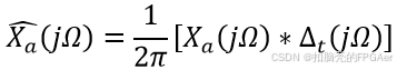
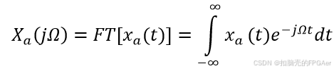
3.2.2 采样序列的频域
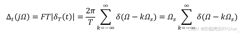
3.2.3 周期性冲激函数序列的频域
这里对于 的计算过程:
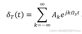
- 周期性冲激函数序列用傅里叶级数展开:
- 傅里叶级数的系数:
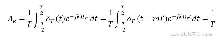
这里 ,
, 称为采样角频率;
 ,
, 称为采样频率
- 综上
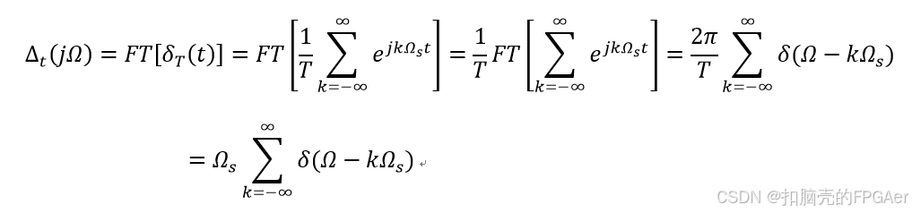
周期冲击函数序列,在频域上是幅度为,谱间隔为的频谱
3.2.4 汇总
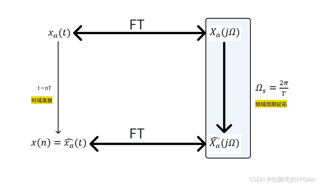
理想采样的频域变换:
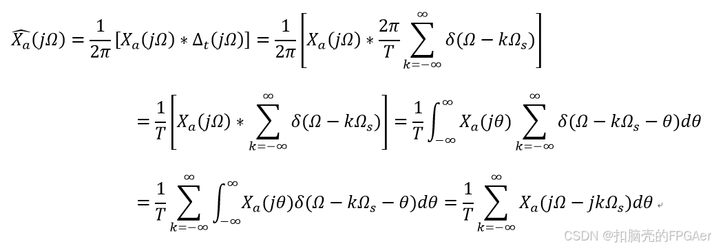
时域离散 <==> 频域周期延拓